Tutorial: Gaussian mixture model and the EM algorithm
MAP573 team
11/10/2020
library(mixtools)Gaussian Mixture Models
We consider a collection of random variables \((X_1, \dots, X_n)\) associated with \(n\) individuals drawn from \(Q\) populations. The label of each individual describes the population (or class) to which it belongs and is unobserved. The \(Q\) classes have a priori distribution \({\boldsymbol \alpha} = (\alpha_1,\dots,\alpha_Q)\) with \(\alpha_q = \mathbb{P}(Z_i = q)\). In other word, the latent variable \(Z_i \in \{1,..,Q\}\) indicating the label follow a multinomial distribution \(Z_i \sim \mathcal{M}(1,\boldsymbol\alpha)\), such as \(\sum_{q=1}^Q \alpha_q = 1\).
The distribution of \(X_i\) conditional on the label of \(i\) is assumed to be a univariate gaussian distribution with unknown parameters, that is, \(X_i | Z_i = q \sim \mathcal{N}(\mu_q,\sigma^2_q)\).
We further introduce the additional notation \(Z_{iq} = \mathbb 1_{\{Z_i = q\}}\) and \(\tau_{iq}= \mathbb{P}(Z_{iq}=1|X_i)\) for posterior probabilities.
We denote the vector of parameters to be estimated by \(\mathbf{\mu} = (\mu_1,\dots,\mu_Q)\), \(\mathbf{\sigma^2} = (\sigma^2_1,\dots,\sigma^2_Q)\), \(\boldsymbol\tau = (\tau_{iq, i=1,\dots,n; q=1,\dots Q})\).
Questions
Likelihood. Write the model complete-data loglikelihood.
E-step. For fixed values of \(\hat{\mu}_q, \hat{\sigma}_{q}^{2}\) and \(\hat\alpha_q\), give the expression of the estimates of the posterior probabilities \(\tau_{iq}= \mathbb{P}(Z_{iq}=1|X_i)\).
M-step. For fixed values of \(\hat{\tau}_{iq}\), show that the maximization step leads to the following estimator for the model parameters: \[ \hat{\alpha}_q = \frac 1n \sum_{i=1}^n \hat{\tau}_{iq}, \:\:\:\:\: \hat{\mu}_q = \frac{\sum_i \hat{\tau}_{iq} x_i}{\sum_i \hat{\tau}_{iq}}, \:\:\:\:\: \hat{\sigma}_q^2 = \frac{\sum_i \hat{\tau}_{iq} (x_i - \hat{\mu}_q)^2}{\sum_i \hat{\tau}_{iq}}. \]
Implementation. Complete the following code.
get_cloglik <- function(X, Z, theta) {
  #returns the complete model loglikelihood
  n <- length(X); Q <- ncol(Z)
  alpha <- theta$alpha; mu <- theta$mu; sigma <- theta$sigma
  Xs <- # to write
  res <- # to write
  res
}

M_step <- function(X, tau) {
  #maximization step
  n <- length(X); Q <- ncol(tau)
  alpha  <- # to write
  mu     <- # to write
  sigma  <- # to write
  list(alpha = alpha, mu = mu, sigma = sigma)
}

E_step <- function(X, theta) {
  #expectation step
  probs <- # to write
  likelihoods <- rowSums(probs)
  list(tau = probs / likelihoods, loglik = sum(log(likelihoods)))
}
EM_mixture <- function(X, Q,
init.cl = base::sample(1:Q, n, rep=TRUE), max.iter=100, eps=1e-5) {
n <- length(X); tau <- matrix(0, n, Q); tau[cbind(1:n, init.cl)] <- 1
loglik <- vector("numeric", max.iter)
Eloglik <- vector("numeric", max.iter)
iter <- 0; cond <- FALSE
while (!cond) {
iter <- iter + 1
## M step
theta <- # to write
## E step
res_Estep <- # to write
tau <- # to write
## check consistency
loglik[iter] <- # to write
Eloglik[iter] <- # to write
if (iter > 1)
cond <- (iter>=max.iter) | Eloglik[iter]-Eloglik[iter-1] < eps
}
res <- list(alpha = theta$alpha, mu = theta$mu, sigma = theta$sigma,
tau = tau, cl = apply(tau, 1, which.max),
Eloglik = Eloglik[1:iter],
loglik = loglik[1:iter])
res
}- Examples. We would like now to assess the performance of our EM algorithm. To do so, we generate:
mu1 <- 5 ; sigma1 <- 1; n1 <- 100
mu2 <- 10 ; sigma2 <- 1; n2 <- 200
mu3 <- 15 ; sigma3 <- 2; n3 <- 50
mu4 <- 20 ; sigma4 <- 3; n4 <- 100
cl <- rep(1:4,c(n1,n2,n3,n4))
x <- c(rnorm(n1,mu1,sigma1),rnorm(n2,mu2,sigma2),
rnorm(n3,mu3,sigma3),rnorm(n4,mu4,sigma4))
n <- length(x)
## we randomize the class ordering
rnd <- base::sample(1:n)
cl <- cl[rnd]
x <- x[rnd]
alpha <- c(n1,n2,n3,n4)/n
curve(alpha[1]*dnorm(x,mu1,sigma1) +
alpha[2]*dnorm(x,mu2,sigma2) +
alpha[3]*dnorm(x,mu3,sigma3) +
alpha[4]*dnorm(x,mu4,sigma3),
col="blue", lty=1, from=0,to=30, n=1000,
main="Theoretical Gaussian mixture and its components",
xlab="x", ylab="density")
curve(alpha[1]*dnorm(x,mu1,sigma1), col="red", add=TRUE, lty=2)
curve(alpha[2]*dnorm(x,mu2,sigma2), col="red", add=TRUE, lty=2)
curve(alpha[3]*dnorm(x,mu3,sigma3), col="red", add=TRUE, lty=2)
curve(alpha[4]*dnorm(x,mu4,sigma4), col="red", add=TRUE, lty=2)
rug(x)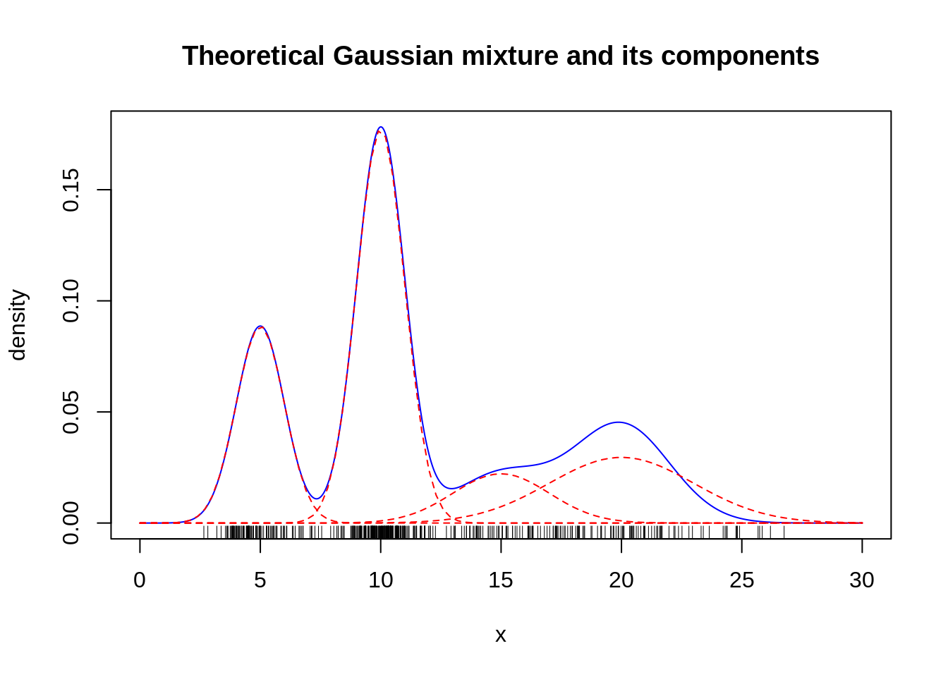 Try your EM algorithm on the simulated data. Comment the results. Consider different initialization. Compare with the output of the function normalmixEm in the package mixtools.
- Model Selection. Discuss the choice of \(Q\) by computing the BIC and ICL criterion and test it on your simulated data. \[ \mathrm{BIC}(Q) = - 2 \log L(X;\hat \alpha, \hat \mu, \hat \sigma^2) +\log(n) \mathrm{df}(Q). \] \[ \mathrm{ICL}(Q) = - 2 \log L(X,Z;\hat \alpha, \hat \mu, \hat \sigma^2) +\log(n) \mathrm{df}(Q). \]