Zero-inflated Normal-Block models: a worked example with fish biomass data

Julien Chiquet & Jeanne Tous

2026-08-07

Preliminaries

This vignette walks through a real-data analysis with the zero-inflated extension of the Normal-Block model, using the onema dataset shipped with the package (see ?onema): fish biomass per species, summed per sampling station, together with environmental covariates. See the normal-block vignette (vignette("normal-block")) for a general introduction to the Normal-Block model on simulated data; this one focuses on what changes when the observations are zero-inflated.

Many entries of onema$biomass are exactly zero: a species simply absent from a given station, not a small positive biomass rounded down. A plain (log-)Normal model cannot represent an excess of exact zeros beyond what its own variance would produce, which biases both the variable-level noise estimates and the inferred clustering. The next section spells out precisely how the zero-inflation extension addresses this; see Tous and Chiquet (2026) for the Normal-Block model itself, and inst/normal_block_models.qmd (the package’s reference card) for the full estimation details.

Mathematical background

The Normal-Block model

The Normal-Block model is a Gaussian latent-variable model for a table of observations $Y \in \mathbb{R}^{n \times p}$ (here, $n$ stations and $p$ species), possibly after correcting for covariates $X \in \mathbb{R}^{n \times d}$ (here, water temperature). Conditionally on $q$ latent factors $W_i \in \mathbb{R}^q$, one per cluster of variables:

$$\begin{aligned} \text{latent space:} \quad & W_i \sim \mathcal{N}(0, \Omega^{-1}) \\ \text{observation space:} \quad & Y_i \mid W_i \sim \mathcal{N}(C W_i + B^\top X_i,\ D) \end{aligned}$$

$C \in \{0,1\}^{p \times q}$ assigns every variable to exactly one of the $q$ clusters; it is either given (known clustering) or, as in this vignette, itself unknown and inferred jointly with everything else, in which case the model carries a variational posterior distribution over $C$ rather than a single point estimate. $D$ is the residual (idiosyncratic) covariance of each variable, taken diagonal here. The key structural assumption is that two variables in the same cluster share the same latent factor: their covariance is driven entirely by $\mathrm{Var}(W_k) = (\Omega^{-1})_{kk}$, a single value for the whole cluster, rather than by a separate pairwise term for every pair of variables. 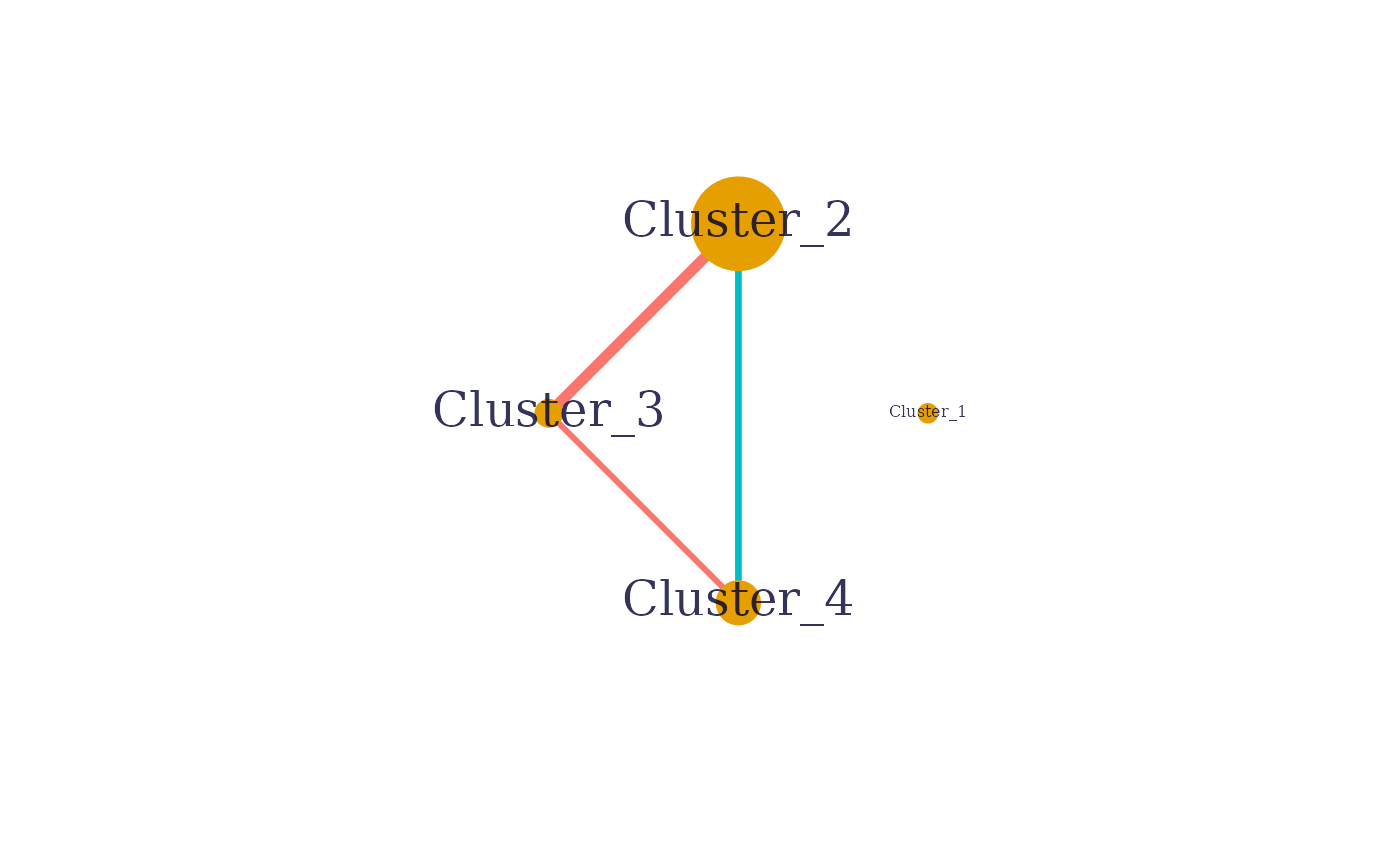$\Omega$, the latent factors’ precision matrix, is what plot_network() displays: the inferred association network between clusters, not between individual species.

Zero-inflation extension

The zero-inflation extension adds an excess-of-zero layer on top of this model. Each observation $Y_{ij}$ is, independently of $W_i$, either a structural zero or a draw from the Normal-Block model above:

$$\begin{aligned} \text{excess-of-zero layer:} \quad & Z_{ij} \sim \mathcal{B}(\kappa_{ij}) \\ \text{observation space:} \quad & Y_i \mid Z_i, W_i = Z_i \odot \mathbf{0} + (1 - Z_i) \odot \big(C W_i + \mathcal{N}(B^\top X_i, D)\big) \end{aligned}$$

so that $\mathbb P(Y_{ij} = 0) \geq \kappa_{ij}$: an excess of zeros beyond what the Normal-Block layer alone would produce, attributed to $Z_{ij} = 1$ (a structural zero) rather than to the (log-)Normal noise.

The zero-inflation probabilities $\kappa$

$\kappa_{ij} = \mathrm{logit}^{-1}(x_{0,i}^\top b_{0,j})$: each variable $j$ has its own logistic regression coefficients $b_{0,j}$ on a zero-inflation design matrix $X_0$ (the X0 argument of NormalBlockData$new()), so $\kappa$ can in general vary across both samples and variables. By default, as in this vignette, X0 is left unspecified and defaults to an intercept-only column: $x_{0,i}$ is then the same constant for every station, so $\kappa_{ij}$ collapses to a single probability per species, $\kappa_j$ – and, since an intercept-only logistic regression’s fitted probability is just the response’s empirical mean, $\kappa_j$ turns out to be exactly that species’ empirical proportion of zeros (checked numerically below). Supplying a non-trivial X0 (e.g. some of the same environmental covariates used in X) would instead let a species’ propensity to be absent vary across stations.

Unlike $B$, $\Omega$ and the clustering, which are refined together by the variational EM recursion below, $\kappa$ (equivalently, $b_0$) is estimated once, upfront, via $p$ independent logistic regressions – it does not change across (V)EM iterations, and so never appears in the optimization trace or convergence plots.

Requirements

library(normalblockr)

The data

data(onema)
dim(onema$biomass)
#> [1] 399  46

onema$biomass is a station-by-species matrix of total biomass (grams); onema$covariates has one row per station, in the same order, with 14 environmental variables. Zero-inflation is the rule here, not the exception:

mean(onema$biomass == 0) # overall
#> [1] 0.7019723
range(colMeans(onema$biomass == 0)) # per-species range
#> [1] 0.2155388 0.9749373

Seven in ten entries are exact zeros, and even the most ubiquitous species is absent from over a fifth of the stations. A histogram of the (log-transformed) data makes the case for zero-inflation visually: a large spike exactly at zero, separate from an otherwise unimodal, roughly bell-shaped distribution of the strictly positive biomasses.

Y_log <- log(1 + onema$biomass)
h <- hist(Y_log, breaks = 50, plot = FALSE)
ymax <- max(h$counts[-1]) * 1.15 # the zero bar (h$counts[1]) dwarfs every other one

plot(h, ylim = c(0, ymax), main = "", xlab = "log(1 + biomass)",
     col = "grey80", border = "white")
arrows(x0 = diff(h$breaks)[1] / 2, y0 = ymax * 0.93, y1 = ymax,
       length = 0.08, angle = 25, col = "grey30", lwd = 2)
text(x = diff(h$breaks)[1], y = ymax * 0.86,
     labels = paste0(round(mean(Y_log == 0) * 100), "% zeros, bar cut off"),
     pos = 4, col = "grey30")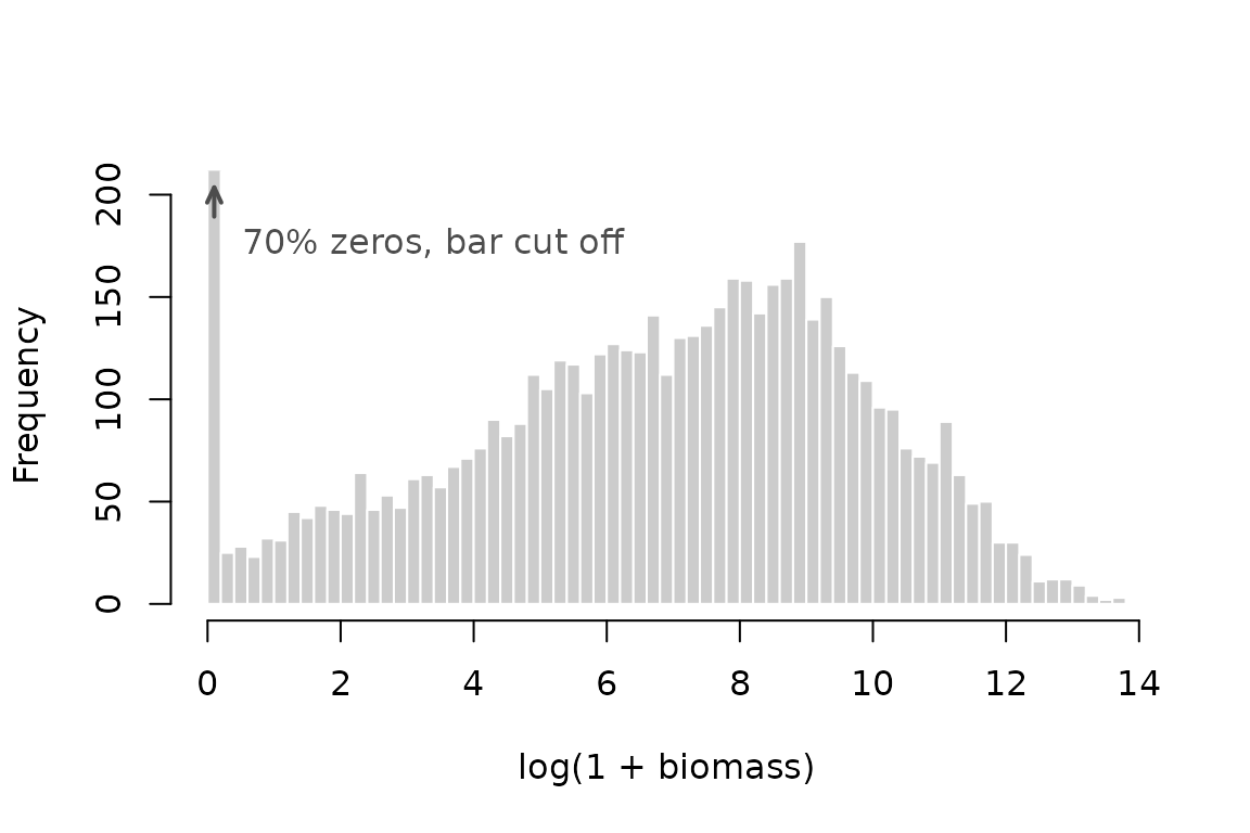

A plain Normal model would have to stretch its variance to accommodate the zero spike as part of the same single Gaussian shape, degrading the fit of the (more informative) positive part. The zero-inflation layer instead lets the spike be absorbed by $\kappa_j$, freeing the Normal-Block model to focus on describing the positive biomasses only.

Preparing the data

As in the general vignette, observations and covariates are wrapped in a NormalBlockData object. We log-transform the (always non-negative) biomass and correct for one covariate, the median water temperature at each station:

X <- model.matrix(~ 1 + temperature_med, data = onema$covariates)
Y <- log(1 + onema$biomass)
data <- NormalBlockData$new(Y, X)

No separate zero-inflation design matrix is supplied here, so NormalBlockData defaults X0 to an intercept-only column: each species gets its own zero-inflation probability $\kappa_j$, estimated independently of the covariates (see ?NormalBlockData to instead let $\kappa$ depend on covariates through X0).

Fitting a zero-inflated Normal-Block model

Everything else works exactly as in the non-zero-inflated case (see the general vignette): the only difference is zero_inflation = TRUE. The number of clusters is rarely known in advance for this kind of data, so we let normal_block explore a range and return a collection of fitted models, one per number of clusters:

out <- normal_block(data, blocks = 2:8, zero_inflation = TRUE)
#> Fitting a diagonal normal-block model with unknown q 
#>   number of blocks = 2                number of blocks = 3                number of blocks = 4                number of blocks = 5                number of blocks = 6                number of blocks = 7                number of blocks = 8           
#> DONE

out$plot(criteria = c("BIC", "EBIC", "deviance"))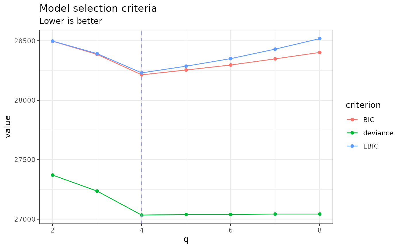

Refining the collection

Each model in the collection above is initialized independently (a heuristic clustering on the zero-inflation-aware residuals, see ?NB_control‘s clustering_init), which can occasionally settle into a milder local optimum than a neighboring number of clusters’ solution would. refine() tries a short split/merge trial from each model’s already-fitted neighbors and keeps it only if it strictly improves – see ?NormalBlockVarCollectionClusters for the full rationale. It is not run by default (it adds real cost), so it is called explicitly here:

out$refine()
#>   refine: q = 3 -- no improvement found ( split )
#>   refine: q = 4 -- no improvement found ( split )
#>   refine: q = 5 -- deviance 27038.71 -> 27034 (improved via split )
#>   refine: q = 6 -- deviance 27038.71 -> 27034 (improved via split )
#>   refine: q = 7 -- deviance 27042.68 -> 27034 (improved via split )
#>   refine: q = 8 -- deviance 27042.68 -> 27034 (improved via split )
#>   refine: q = 7 -- no improvement found ( merge )
#>   refine: q = 6 -- no improvement found ( merge )
#>   refine: q = 5 -- no improvement found ( merge )
#>   refine: q = 4 -- no improvement found ( merge )
#>   refine: q = 3 -- deviance 27235.92 -> 27096.47 (improved via merge )
#>   refine: q = 2 -- deviance 27370.52 -> 27261.14 (improved via merge )
out$plot(criteria = c("BIC", "EBIC", "deviance"))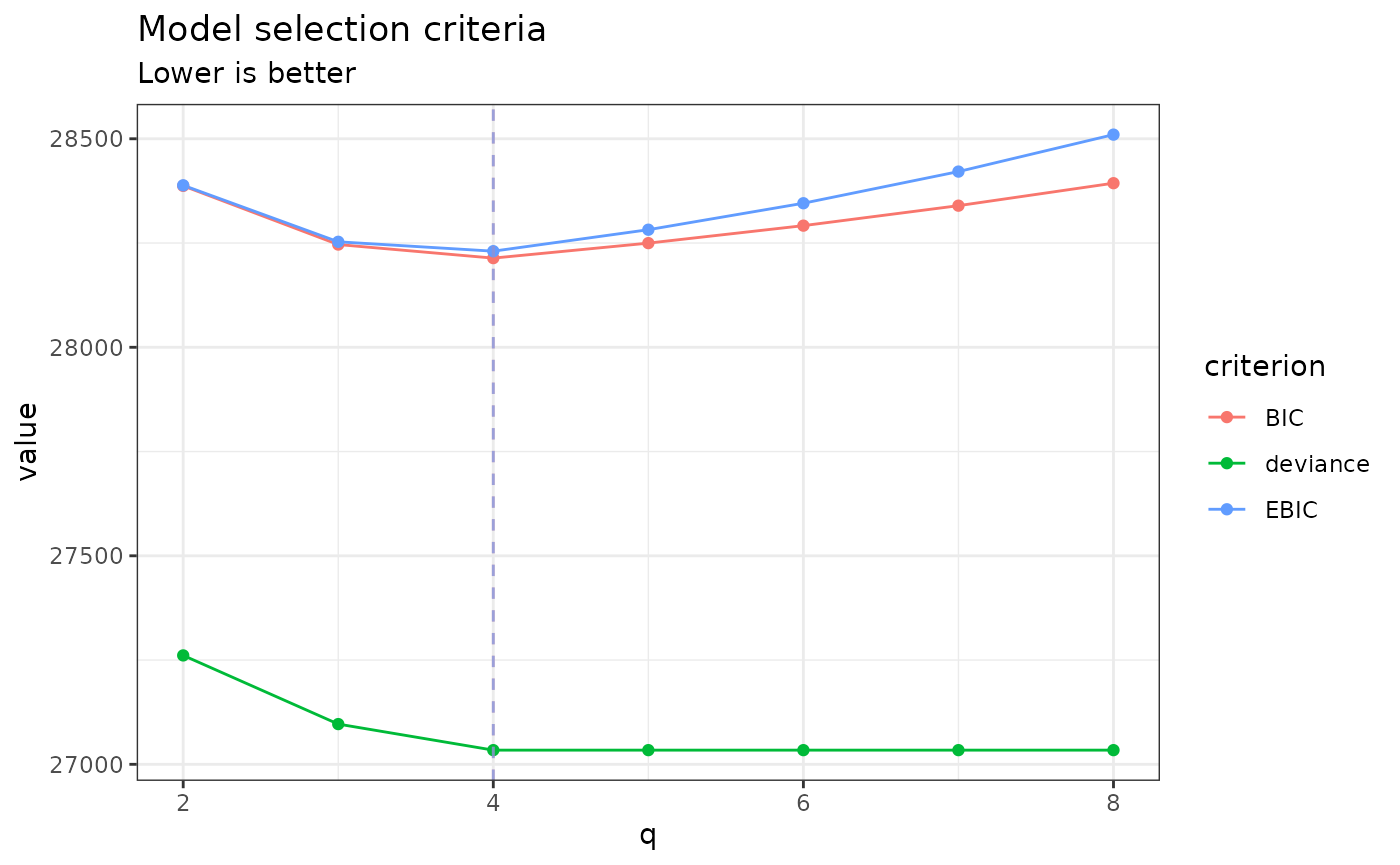

Selecting a model and inspecting the clustering

As with non-zero-inflated collections, a specific model is retrieved with get_model() (by number of clusters) or get_best_model() (by criterion):

myModel <- out$get_best_model("EBIC")
myModel$q
#> [1] 4

elements_per_cluster lists, for each inferred block, the species it groups together:

myModel$elements_per_cluster
#> $`1`
#> [1] "TAC" "TRF" "ANG" "GRE" "OBR"
#> 
#> $`2`
#>  [1] "GAR" "CCO" "TAN" "BRO" "CAS" "LOR" "PER" "ABL" "ROT" "BRB" "BRE" "BOU"
#> [13] "SAN" "PES" "PCH" "PSR" "SIL" "ABH" "IDE" "TOX" "BBG" "GAM" "GOX"
#> 
#> $`3`
#> [1] "GOU" "VAN" "CHE" "BAF" "HOT" "SPI" "VAR"
#> 
#> $`4`
#>  [1] "EPI" "LOF" "CHA" "LPP" "VAI" "EPT" "LOT" "BLN" "PHX" "GOO" "BAM"

Inspecting the zero-inflation probabilities

The fitted zero-inflation probabilities are available through model_par$kappa: an $n \times p$ matrix in general (one $\kappa_{ij}$ per station/species pair), but here, with the intercept-only X0 used above, every row is identical – one probability per species, $\kappa_j$:

kappa_hat <- myModel$model_par$kappa[1, ]
range(kappa_hat)
#> [1] 0.2155388 0.9749373

As explained above, this $\kappa_j$ is exactly that species’ empirical proportion of zeros:

all.equal(kappa_hat, colMeans(onema$biomass == 0), check.attributes = FALSE)
#> [1] TRUE

A species’ zero-inflation probability is not a nuisance parameter to discard: it is a direct estimate of how often that species is structurally absent from a station, as opposed to merely caught in small quantity. The most and least zero-inflated species here illustrate the range:

sort(round(kappa_hat, 2), decreasing = TRUE)[1:5] # almost always structurally absent
#> self.data.X0 self.data.X0 self.data.X0 self.data.X0 self.data.X0 
#>         0.97         0.97         0.97         0.96         0.94
sort(round(kappa_hat, 2))[1:5]                    # almost always present in some quantity
#> self.data.X0 self.data.X0 self.data.X0 self.data.X0 self.data.X0 
#>         0.22         0.23         0.24         0.26         0.32

Sparsifying the association network

Once a number of clusters is chosen, the same sparsity options as in the non-zero-inflated case apply: fitting at the selected q with sparsity = TRUE explores a path of $\ell_1$ penalties on the inter-cluster association network (see Tous and Chiquet 2026).

out_sp <- normal_block(data, blocks = myModel$q, sparsity = TRUE, zero_inflation = TRUE)
#> Fitting a Collection of  zero-inflated diagonal normal-block models with fixed q, with different sparsity penalties. 
#>   penalty = 0.03319511                penalty = 0.028321              penalty = 0.02416257                penalty = 0.02061473                penalty = 0.01758782                penalty = 0.01500536                penalty = 0.01280209                penalty = 0.01092234                penalty = 0.009318585               penalty = 0.007950317               penalty = 0.006782955               penalty = 0.005786999               penalty = 0.004937282               penalty = 0.00421233                penalty = 0.003593825               penalty = 0.003066136               penalty = 0.002615928               penalty = 0.002231826               penalty = 0.001904122               penalty = 0.001624536               penalty = 0.001386002               penalty = 0.001182492               penalty = 0.001008864               penalty = 0.0008607306              penalty = 0.0007343476              penalty = 0.0006265218              penalty = 0.0005345283              penalty = 0.0004560423              penalty = 0.0003890807              penalty = 0.0003319511           
#> DONE
out_sp$plot(c("BIC", "EBIC"))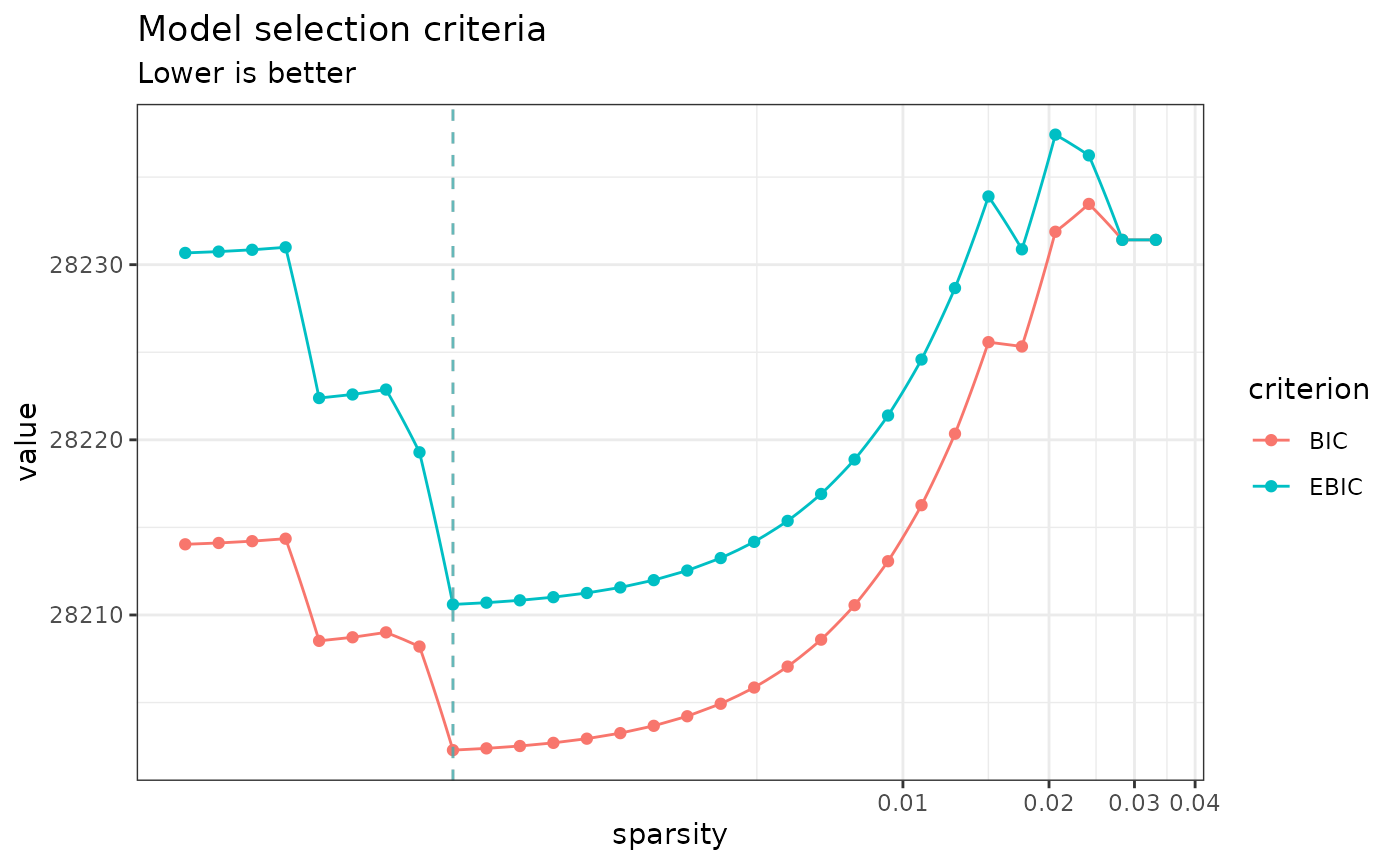

out_sp$plot(c("ICL", "deviance"))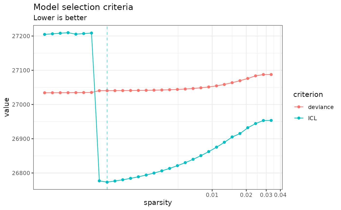

Unlike deviance, which decreases monotonically as the penalty relaxes (a less penalized network is always at least as expressive), BIC/EBIC can bump up locally along the path: each extra edge costs a fixed log(n) in the parameter-count penalty, and whenever its actual gain in deviance is smaller than that, the criterion increases even though both the deviance and the parameter count keep moving in the expected direction. This is the intended behavior of a penalized criterion, not a bug in the parameter count.

The association network at the best ICL penalty can then be visualized directly:

out_sp$get_best_model("ICL")$plot_network()

References

Tous, Jeanne, and Julien Chiquet. 2026. “An Integrated Method for Clustering and Association Network Inference.” Computational Statistics & Data Analysis 219: 108347. https://doi.org/10.1016/j.csda.2026.108347.