Normal-Block models: a worked example with breast cancer proteomics data

Preliminaries

This vignette walks through a real-data analysis with the Normal-Block model, using the brca_rppa dataset shipped with the package (see ?brca_rppa): reverse-phase protein array measurements of 163 proteins across 346 breast cancer tumor samples from The Cancer Genome Atlas, together with each sample’s PAM50 molecular subtype. See the normal-block vignette (vignette("normal-block")) for a general introduction to the package on simulated data; this one focuses on a single real dataset, illustrated first with a known clustering of the proteins, then with the clustering left for the model to infer, and finally with the post-hoc refine() step.

This dataset is also the running example of Tous and Chiquet (2026), which includes a biological-enrichment analysis of the inferred clusters (enrichKEGG/compareCluster, via clusterProfiler) – not reproduced here, since it pulls in several heavy Bioconductor dependencies and network queries; see inst/CSDA_analyses/analysis_breast_cancer_proteomics.qmd in the package sources for the full analysis, enrichment included.

Requirements

library(normalblockr)

Mathematical background

The Normal-Block model is a Gaussian latent-variable model for a table of observations $Y \in \mathbb{R}^{n \times p}$ (here, $n$ tumor samples and $p$ proteins), possibly after correcting for covariates $X \in \mathbb{R}^{n \times d}$ (here, the PAM50 subtype). Conditionally on $q$ latent factors $W_i \in \mathbb{R}^q$ , one per cluster of variables:

$\begin{aligned} \text{latent space:} \quad & W_i \sim \mathcal{N}(0, \Omega^{-1}) \\ \text{observation space:} \quad & Y_i \mid W_i \sim \mathcal{N}(C W_i + B^\top X_i,\ D) \end{aligned}$

$C \in \{0,1\}^{p \times q}$ assigns every protein to exactly one of the $q$ clusters; it is either given (known clustering, e.g. from an independent source) or itself unknown and inferred jointly with everything else, in which case the model carries a variational posterior distribution over $C$ rather than a single point estimate. $D$ is the residual (idiosyncratic) covariance of each protein, taken diagonal here. The key structural assumption is that two proteins in the same cluster share the same latent factor: their covariance is driven entirely by $\mathrm{Var}(W_k) = (\Omega^{-1})_{kk}$ , a single value for the whole cluster, rather than by a separate pairwise term for every pair of proteins. 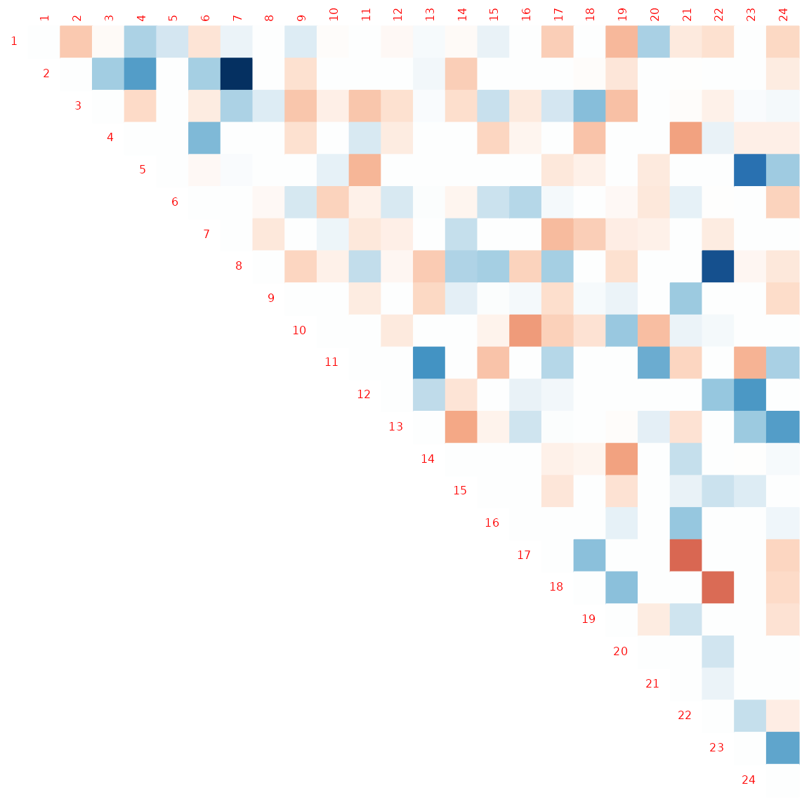$\Omega$ , the latent factors’ precision matrix, is what plot_network() displays: the inferred association network between clusters, not between individual proteins. In its plain (non-regularized) form, that network is dense and not very informative to look at directly – we only visualize it at the end of this vignette, after regularizing it with a graphical lasso penalty (section 10 of inst/normal_block_models.qmd).

See Tous and Chiquet (2026) for the model itself, and inst/normal_block_models.qmd (the package’s reference card) for the full estimation details (criteria, E/M updates, and the accelerated variational EM recursion used to fit it).

The data

data(brca_rppa)
dim(brca_rppa$expr)
#> [1] 346 163
table(brca_rppa$covariates$PAM50_SUBTYPE)
#> 
#>    Basal-like HER2-enriched     Luminal A     Luminal B   Normal-like 
#>            66            43           150            82             5

expr is the $346 \times 163$ matrix of (samples x proteins) expression levels; the PAM50 subtype, a 5-level clinical covariate, is used as $X$ throughout, so that the model accounts for each subtype’s own mean expression level before looking for structure in what’s left.

Y            <- as.matrix(brca_rppa$expr)
X_subtype    <- model.matrix(~ 0 + PAM50_SUBTYPE, data = brca_rppa$covariates)
data_subtype <- NormalBlockData$new(Y, X_subtype)

A known clustering of the proteins

Before letting the Normal-Block model infer its own grouping of the proteins, we build a simple, fully data-driven baseline: a hierarchical (Ward) clustering of the proteins from their expression profiles alone, with no reference to the Normal-Block model at all. By default normalblockr scales the data, so this a priori clustering is computed on the same (column-)scaled matrix for consistency. Six clusters is an arbitrary but visually natural cut of the dendrogram.

hc_expr <- brca_rppa$expr |> scale() |> t() |> dist() |> hclust("ward.D2")
plot(hc_expr, labels = FALSE, hang = -1,
     main = "Hierarchical clustering of proteins (Ward, on scaled expression)",
     xlab = "proteins", sub = "")
rect.hclust(hc_expr, k = 6, border = "red")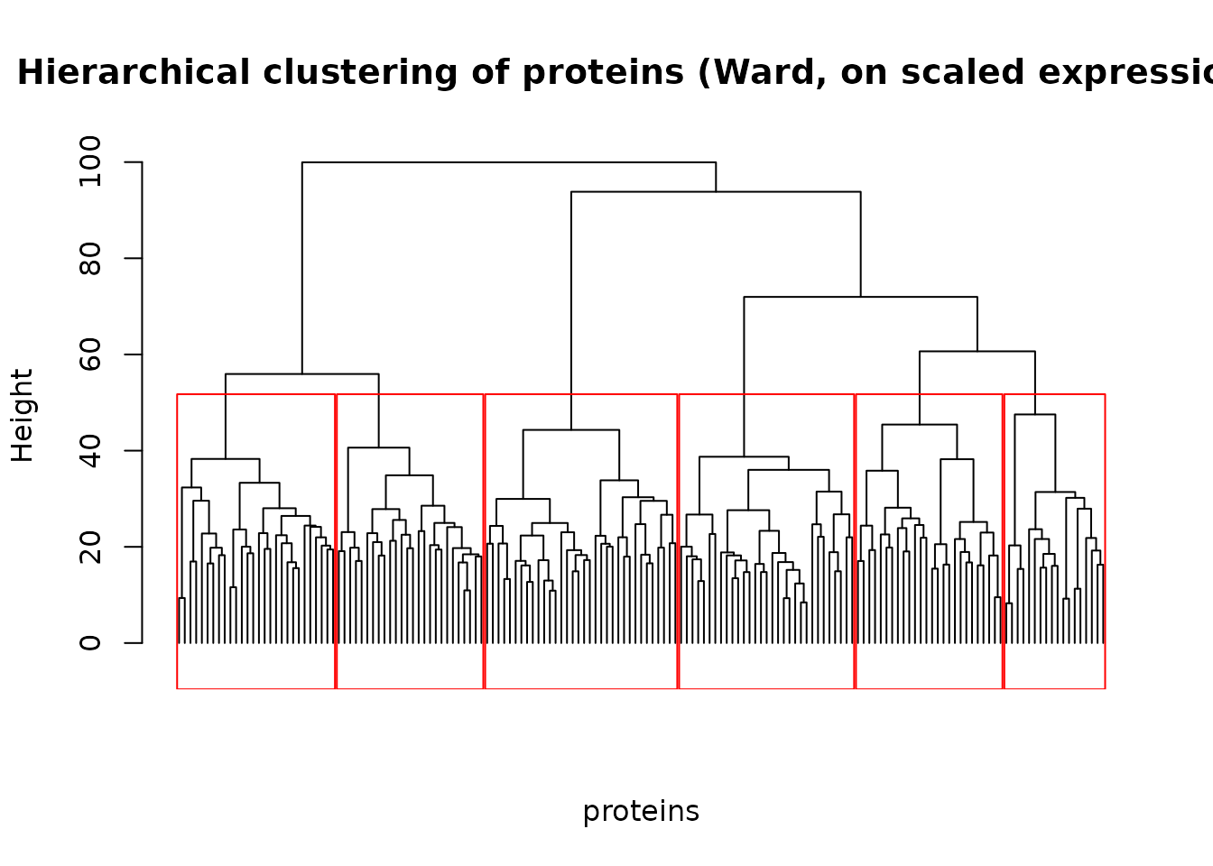

group <- cutree(hc_expr, 6) |> normalblockr:::as_indicator()

This fixed grouping is then handed to normal_block() as a known clustering – the model only estimates the association network between the 6 blocks, not the grouping itself.

NB_prot_group <- normal_block(data_subtype, blocks = group)
#> Fitting a diagonal normal-block model with fixed blocks 
#> 
#> DONE
plot(NB_prot_group)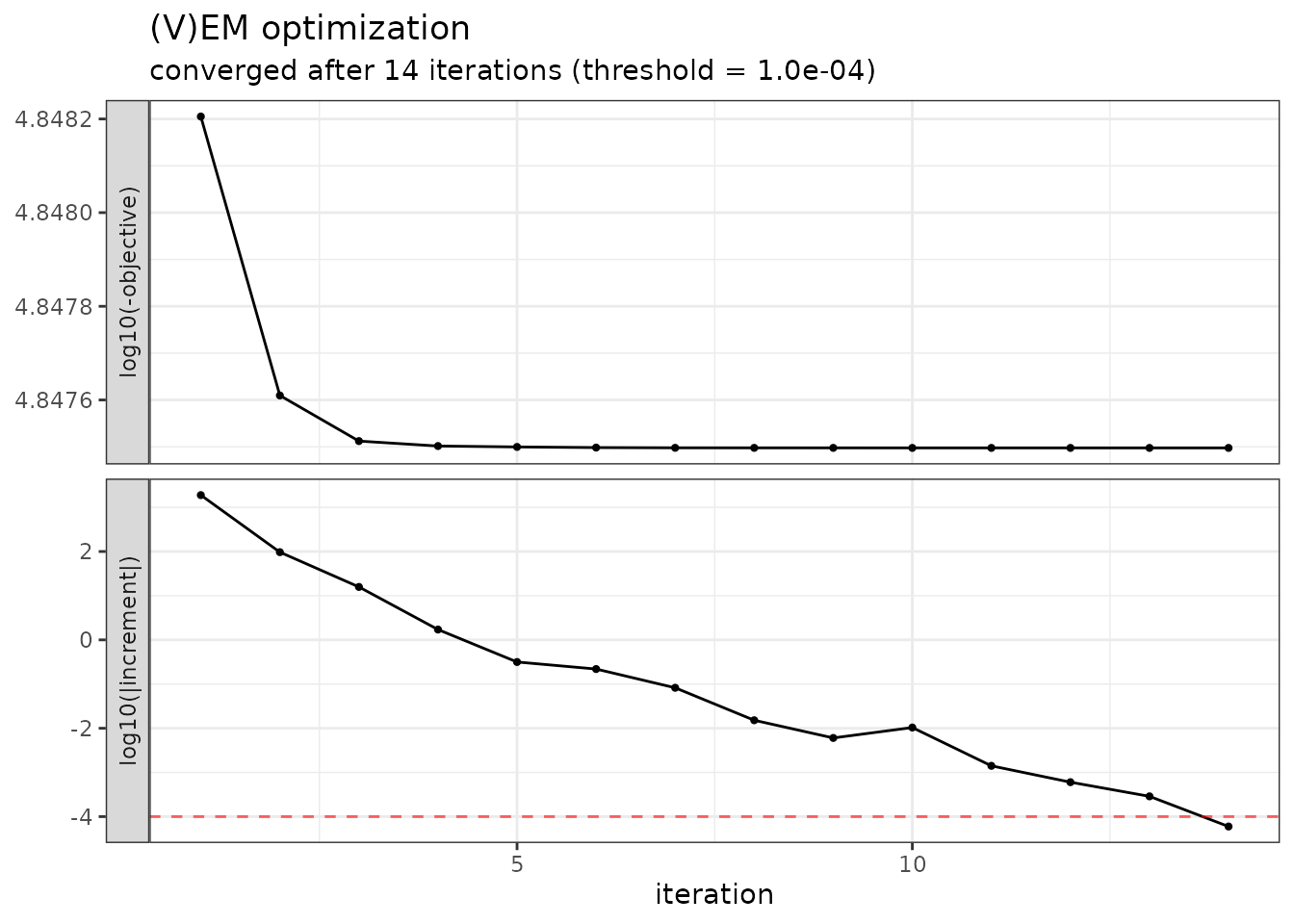

print(NB_prot_group)
#> A diagonal normal-block model with fixed blocks .
#> ===========================================================================
#>  nb_param q n_edges sparsity    loglik deviance      BIC      ICL   EBIC niter
#>       999 6      15        0 -70387.84 140775.7 146616.3 144073.3 146670    14
#> ===========================================================================
#> * Useful fields
#>     $model_par, $posterior_par / $var_par, $clustering 
#>     $loglik, $BIC, $ICL, $objective, $nb_param, $criteria
#> * Useful S3 methods
#>     print(), summary(), plot(), coef(), sigma(), fitted(), predict()

Letting the model infer its own clustering

Fitting a collection over a range of cluster counts

When the clustering is left unknown, normal_block() accepts a range of candidate cluster counts and returns a collection of models, one per $q$ , fitted independently, each cold-started from a clustering heuristic on the residuals (ward2 by default). Different heuristics can converge to substantially different (V)EM local optima at the same $q$ ; NB_control(clustering_init = "best_of_inits") tries several and keeps the best-ELBO fit, at extra cost – worth it when refine() (next section) won’t also be applied, but on this dataset’s full range refine() alone already recovers most of what it would add (see inst/clustering_initialization_benchmark), so we stick with the default here.

NB_prot_subtype <- normal_block(data_subtype, blocks = 1:30)
#> Fitting a diagonal normal-block model with unknown q 
#>   number of blocks = 1                number of blocks = 2                number of blocks = 3                number of blocks = 4                number of blocks = 5                number of blocks = 6                number of blocks = 7                number of blocks = 8                number of blocks = 9                number of blocks = 10               number of blocks = 11               number of blocks = 12               number of blocks = 13               number of blocks = 14               number of blocks = 15               number of blocks = 16               number of blocks = 17               number of blocks = 18               number of blocks = 19               number of blocks = 20               number of blocks = 21               number of blocks = 22               number of blocks = 23               number of blocks = 24               number of blocks = 25               number of blocks = 26               number of blocks = 27               number of blocks = 28               number of blocks = 29               number of blocks = 30           
#> DONE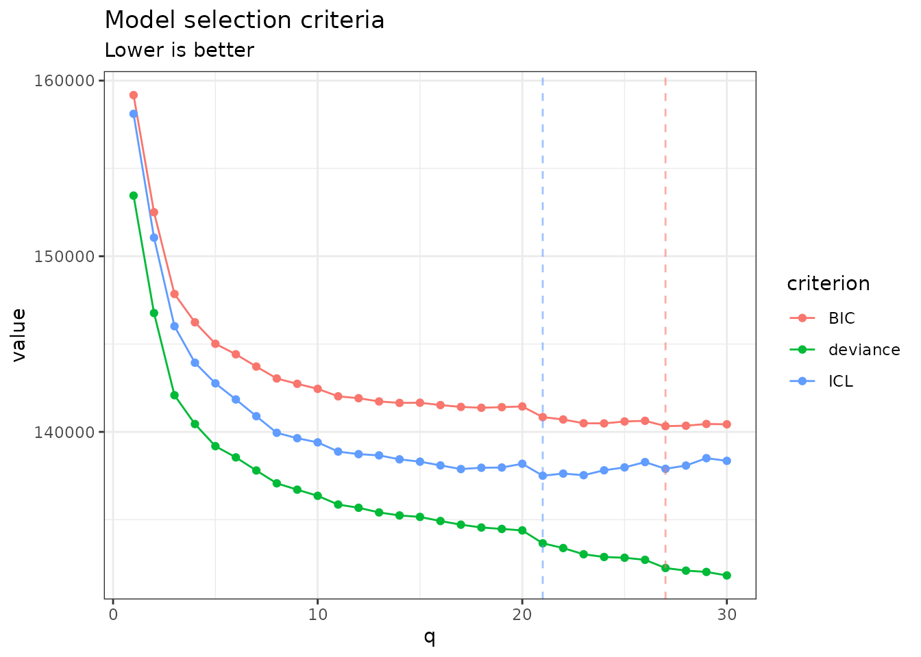

Model selection: criteria to fix the number of clusters

NB_prot_subtype$plot(c("deviance", "BIC", "ICL"))

selected_NB <- NB_prot_subtype$get_best_model("ICL")
paste0("ICL selects ", selected_NB$q, " clusters.")
#> [1] "ICL selects 21 clusters."

Refining the clustering

Every model in the collection above was fitted independently, cold-started from its own clustering heuristic – which, on real data, can settle into a milder local optimum than an incremental, neighbor-seeded search would. refine() tries, for every $q$ beyond the collection’s extremes, a short split-and-reoptimize trial seeded from its already-fitted $q-1$ neighbor and/or a short merge-and-reoptimize trial seeded from its $q+1$ neighbor, keeping a candidate only if it strictly improves the deviance. It runs unconditionally over the whole range and discards whatever doesn’t help, so it can only improve (or leave unchanged) each model it touches.

NB_prot_subtype$refine()
#>   refine: q = 2 -- no improvement found ( split )
#>   refine: q = 3 -- no improvement found ( split )
#>   refine: q = 4 -- no improvement found ( split )
#>   refine: q = 5 -- no improvement found ( split )
#>   refine: q = 6 -- deviance 138548.1 -> 138420.2 (improved via split )
#>   refine: q = 7 -- no improvement found ( split )
#>   refine: q = 8 -- deviance 137071.8 -> 137054.2 (improved via split )
#>   refine: q = 9 -- deviance 136709.9 -> 136505.3 (improved via split )
#>   refine: q = 10 -- deviance 136359.2 -> 136240.6 (improved via split )
#>   refine: q = 11 -- no improvement found ( split )
#>   refine: q = 12 -- deviance 135679.5 -> 135565.1 (improved via split )
#>   refine: q = 13 -- deviance 135413.1 -> 135345.5 (improved via split )
#>   refine: q = 14 -- deviance 135242.5 -> 135206.2 (improved via split )
#>   refine: q = 15 -- deviance 135159 -> 135012.8 (improved via split )
#>   refine: q = 16 -- deviance 134925.2 -> 134839.3 (improved via split )
#>   refine: q = 17 -- no improvement found ( split )
#>   refine: q = 18 -- no improvement found ( split )
#>   refine: q = 19 -- no improvement found ( split )
#>   refine: q = 20 -- deviance 134390.4 -> 134268.2 (improved via split )
#>   refine: q = 21 -- no improvement found ( split )
#>   refine: q = 22 -- no improvement found ( split )
#>   refine: q = 23 -- no improvement found ( split )
#>   refine: q = 24 -- deviance 132876.8 -> 132819 (improved via split )
#>   refine: q = 25 -- deviance 132833.9 -> 132535.9 (improved via split )
#>   refine: q = 26 -- deviance 132714.6 -> 132325.5 (improved via split )
#>   refine: q = 27 -- deviance 132248.1 -> 132229 (improved via split )
#>   refine: q = 28 -- no improvement found ( split )
#>   refine: q = 29 -- deviance 132026 -> 131886.7 (improved via split )
#>   refine: q = 30 -- deviance 131826.3 -> 131590 (improved via split )
#>   refine: q = 29 -- deviance 131886.7 -> 131710.5 (improved via merge )
#>   refine: q = 28 -- deviance 132100.6 -> 131695.1 (improved via merge )
#>   refine: q = 27 -- deviance 132229 -> 131790.6 (improved via merge )
#>   refine: q = 26 -- deviance 132325.5 -> 132006.9 (improved via merge )
#>   refine: q = 25 -- deviance 132535.9 -> 132101.8 (improved via merge )
#>   refine: q = 24 -- deviance 132819 -> 132245.4 (improved via merge )
#>   refine: q = 23 -- deviance 133032.2 -> 132559.2 (improved via merge )
#>   refine: q = 22 -- deviance 133386.1 -> 132775.6 (improved via merge )
#>   refine: q = 21 -- deviance 133657 -> 133100.4 (improved via merge )
#>   refine: q = 20 -- deviance 134268.2 -> 133304.7 (improved via merge )
#>   refine: q = 19 -- deviance 134474 -> 133535.5 (improved via merge )
#>   refine: q = 18 -- deviance 134556 -> 133736 (improved via merge )
#>   refine: q = 17 -- deviance 134716 -> 133957.3 (improved via merge )
#>   refine: q = 16 -- deviance 134839.3 -> 134173.3 (improved via merge )
#>   refine: q = 15 -- deviance 135012.8 -> 134382.5 (improved via merge )
#>   refine: q = 14 -- deviance 135206.2 -> 134480.5 (improved via merge )
#>   refine: q = 13 -- deviance 135345.5 -> 134828.3 (improved via merge )
#>   refine: q = 12 -- deviance 135565.1 -> 135178.5 (improved via merge )
#>   refine: q = 11 -- deviance 135862.7 -> 135468 (improved via merge )
#>   refine: q = 10 -- deviance 136240.6 -> 135901.9 (improved via merge )
#>   refine: q = 9 -- deviance 136505.3 -> 136405.7 (improved via merge )
#>   refine: q = 8 -- deviance 137054.2 -> 136976.7 (improved via merge )
#>   refine: q = 7 -- deviance 137802.5 -> 137699.4 (improved via merge )
#>   refine: q = 6 -- no improvement found ( merge )
#>   refine: q = 5 -- no improvement found ( merge )
#>   refine: q = 4 -- no improvement found ( merge )
#>   refine: q = 3 -- deviance 142087.1 -> 142081 (improved via merge )
#>   refine: q = 2 -- no improvement found ( merge )
#>   refine: q = 1 -- no improvement found ( merge )

NB_prot_subtype$plot(c("deviance", "BIC", "ICL"))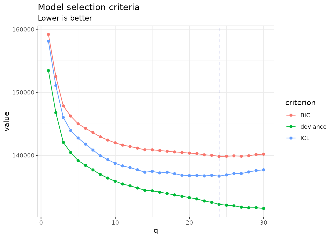

selected_NB_refined <- NB_prot_subtype$get_best_model("ICL")
paste0("After refine(), ICL selects ", selected_NB_refined$q, " clusters.")
#> [1] "After refine(), ICL selects 24 clusters."

On this dataset, refine() moves the ICL-selected number of clusters – a reminder that the collection-wide local search is not just cosmetic: a clustering that looked locally optimal in isolation can still be improved once its neighbors in $q$ are available as alternative starting points.

Sparsifying the network of the selected clustering

The association network $\Omega$ of the ICL-selected model above is dense (no penalty was applied), which makes it hard to read directly. Treating that clustering as fixed, we can refit the model once more with the graphical-lasso penalty on $\Omega$ explored over a path of values (sparsity = TRUE, see section 10 of inst/normal_block_models.qmd), and pick the sparsity level with the best BIC.

group_selected <- selected_NB_refined$clustering |> normalblockr:::as_indicator()
NB_prot_sparse <- normal_block(data_subtype, blocks = group_selected, sparsity = TRUE, control = NB_control(min_ratio=0.001))
#> Fitting a Collection of diagonal normal-block models with fixed blocks, with different sparsity penalties. 
#>   penalty = 0.6628733             penalty = 0.5223748             penalty = 0.4116555             penalty = 0.3244036             penalty = 0.2556451             penalty = 0.2014601             penalty = 0.1587599             penalty = 0.1251102             penalty = 0.0985926             penalty = 0.07769553                penalty = 0.06122767                penalty = 0.04825024                penalty = 0.03802342                penalty = 0.02996422                penalty = 0.02361319                penalty = 0.01860829                penalty = 0.01466419                penalty = 0.01155606                penalty = 0.009106711               penalty = 0.00717651                penalty = 0.005655422               penalty = 0.004456734               penalty = 0.003512113               penalty = 0.002767707               penalty = 0.002181081               penalty = 0.001718793               penalty = 0.001354489               penalty = 0.0010674             penalty = 0.0008411603              penalty = 0.0006628733           
#> DONE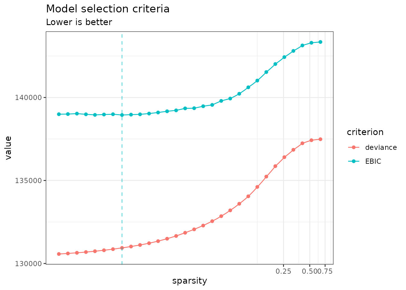

plot(NB_prot_sparse, c("EBIC", "deviance"))

sparse_best <- NB_prot_sparse$get_best_model("EBIC")
paste0("BIC selects a penalty of ", round(sparse_best$sparsity, 4), ".")
#> [1] "BIC selects a penalty of 0.0035."

sparse_best$plot_network(output = "corrplot")

References

Tous, Jeanne, and Julien Chiquet. 2026. “An Integrated Method for Clustering and Association Network Inference.” Computational Statistics & Data Analysis 219: 108347. https://doi.org/10.1016/j.csda.2026.108347.

Julien Chiquet & Jeanne Tous

2026-08-07