Analyzing multivariate Gaussian data with the Normal-Block model (variance clustering) - First steps
Jeanne Tous and Julien Chiquet
2026-10-07
Source:vignettes/normal-block.Rmd
normal-block.RmdPreliminaries
This vignette illustrates the use of the normal_block()
function and the methods accompanying its R6 classes.
From a statistical point of view, the normal_block()
function fits a multivariate Normal-Block model (a Gaussian graphical
model with a latent clustering structure) to a table of observations,
possibly after correcting for the effect of covariates. Depending on the
arguments given, the function uses a clustering supplied by the user or
infers one, includes zero-inflation or not, infers a sparse network or
not, and so on. Parameter inference can either be done with an
integrated variational Expectation-Maximization approach (recommended)
or with a faster heuristic approach.
This vignette covers the default family, where the clustering
structures the covariance of the variables
(model = "var"). A complementary family clusters variables
by their response to covariates instead
(model = "mean"); see
vignette("mean-block-breast-cancer").
Theoretical explanations for this model and full estimation details (criteria, E/M updates) can be found in Tous and Chiquet (2026).
Requirements
library(normalblockr)
library(pheatmap)
library(paletteer)
Data simulation
We illustrate the analysis with two simulated datasets.
Fix the seed to make the results reproducible.
set.seed(1)Simulate data with generate_normal_block_data().
Fix simulation parameters
Several parameters need to be defined to simulate the data:
n = 100 # Number of samples (number of rows in the matrix of observations)
p = 40  # Number of entities observed (number of columns in the matrix of observations)
d = 2   # Number of covariates
q = 3   # Number of clusters
kappa = 0 # Mean zero-inflation probability (can also be a vector to define one ZI-probability for each variable). kappa = 0 means that there is no zero-inflation.
omega_structure = "erdos-renyi" # Network structure.
u_v = c(0.3, 0.1) # Parameters to generate an association matrix from a graph, details given in the bibliography.
SNR = 0.75 # Signal to Noise Ratio, defines the relative weight of the covariates and the variance
alpha = rep(1/q, q) # Vector giving probabilities of belonging to each cluster
range_X = c(0, 10)  # Min and max values for the covariates
range_D = c(0.5, 1.5) # Min and max values for the individual entities variances
Simulation 1 (no zero-inflation)
generate_normal_block_var_data() generates data under
the Normal-Block model. It returns a list containing the simulated
covariates
and observations
,
and the simulation parameters (including the clustering
).
my_nb_data <- generate_normal_block_var_data(n, p, d, q, kappa, omega_structure, u_v,
                                            SNR, alpha, range_X, range_D)
pheatmap::pheatmap(my_nb_data$Y,
                   color =paletteer::paletteer_c("ggthemes::Orange-Gold", n = 100), cluster_rows = FALSE, cluster_cols = FALSE, show_rownames = FALSE)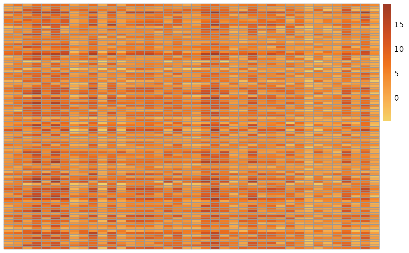
Simulation 2 (with zero-inflation)
To generate zero-inflated data, we set-up kappa as a vector of zero-inflation probabilities. One needs to ensure that these values are between 0 and 1.
kappa_zi <- rnorm(p, mean = 0.7, sd = 0.05)
kappa_zi <- unlist(lapply(kappa_zi, f <- function(x) return(max(0, min(x, 0.9)))))
my_nb_data_zi <- generate_normal_block_var_data(n = n, p = p, d = d, q = 5, kappa = kappa_zi,
                                                omega_structure = omega_structure, u_v = u_v,
                                                SNR = SNR, alpha = alpha,
                                                range_X = range_X, range_D = range_D)
For a better visualization of the zero-inflated data, we set-up the 0 to be shown in white.
min_val <- min(my_nb_data_zi$Y) ; max_val <- max(my_nb_data_zi$Y)
orange_gold_pal <- paletteer::paletteer_c("ggthemes::Orange-Gold", n = 100)
n_breaks <- 100
zero_pos <- round((0 - min_val) / (max_val - min_val) * n_breaks) + 1
custom_pal <- c(orange_gold_pal[1:(zero_pos - 1)], "white", orange_gold_pal[zero_pos:n_breaks])
pheatmap::pheatmap(my_nb_data_zi$Y,
                   color = custom_pal,
                   cluster_rows = FALSE, cluster_cols = FALSE,
                   show_rownames = FALSE)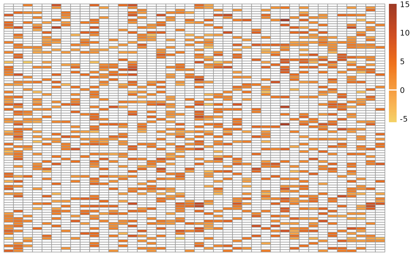
Prepare the data for a Normal-Block analysis
A specific data object of class NormalBlockData needs to
be created to analyse the data with normalblockr.
One can use
and
alone to create the NormalBlockData object.
my_data    <- NormalBlockData$new(my_nb_data$Y, my_nb_data$X)
my_data_zi <- NormalBlockData$new(my_nb_data_zi$Y, my_nb_data_zi$X)
Alternatively, if one only wants to include some of the covariates contained in , a formula can be used to specify which one:
colnames(my_data$X) <- c("X1", "X2")
my_data_alt    <- NormalBlockData$new(my_data$Y, my_data$X, formula = ~ 0 + X1)
Run a Normal-Block analysis
All Normal-Block analyses are run with the
normal_block() function, called with different arguments
depending on whether the clustering (or the number of clusters) is
known, and on the requested level of sparsity, among other factors. See
?normal_block for full details.
By default, the parameters are inferred using a variational
Expectation-Maximization approach, with up to 500 iterations. Finer
control of the optimization is possible through the control
argument of normal_block(), a list generated by
NB_control().
With non-zero-inflated data
Fixed clustering
When the variables’ clustering is known, it can be given directly as
an input to normal_block().
my_NB <- normal_block(data = my_data,
                      blocks = my_nb_data$parameters$C)
#> Fitting a diagonal normal-block-var model with fixed blocks
#>
#> DONE
Convergence of the model can be checked with plot().
plot(my_NB)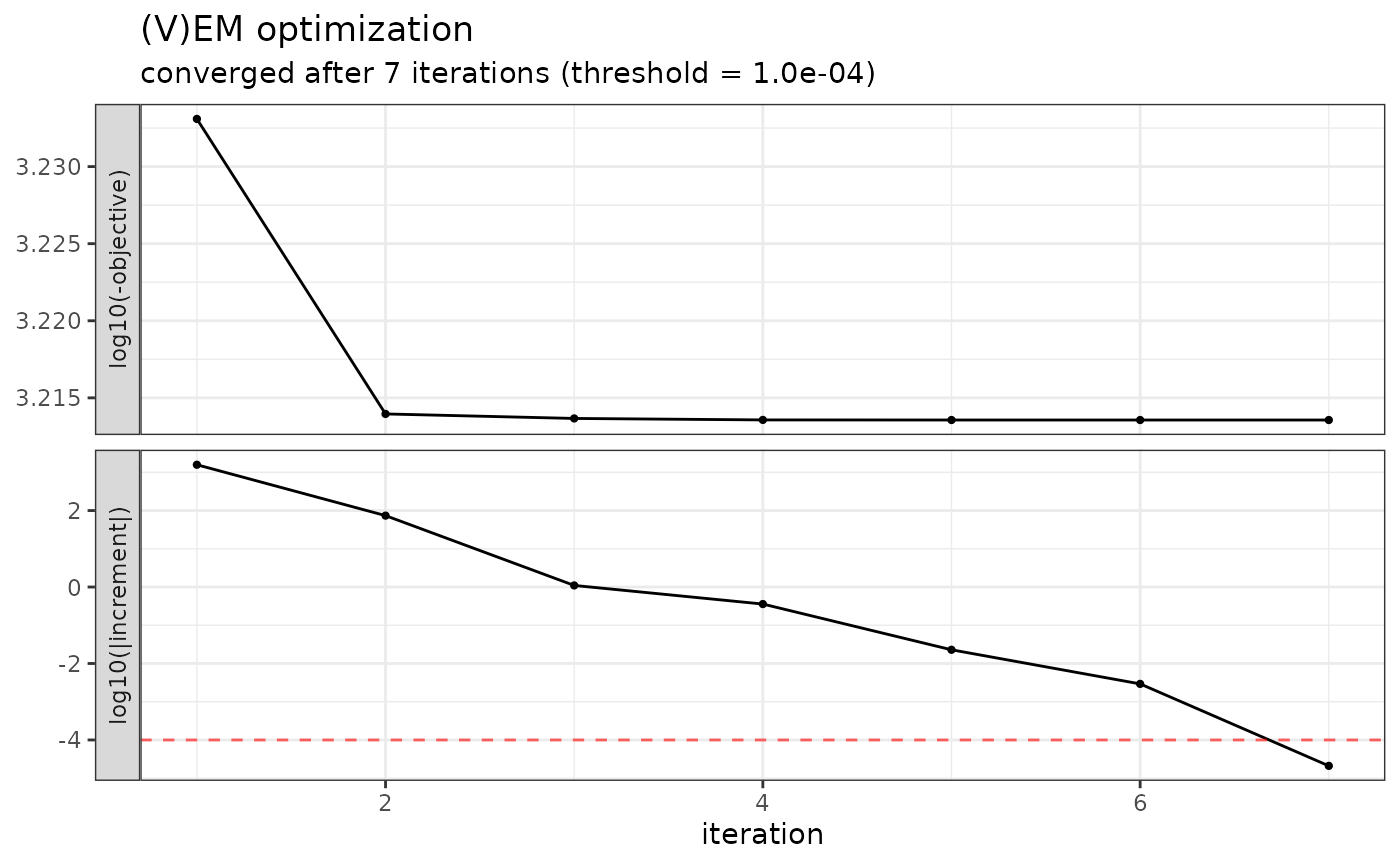
A summary of the results is accessible via print().
print(my_NB)
#> A diagonal normal-block-var model with fixed blocks .
#> ===========================================================================
#>  nb_param q n_edges sparsity   loglik deviance      BIC      ICL     EBIC niter
#>       126 3       3        0 -1635.17  3270.34 3850.592 3198.393 3857.183     7
#> ===========================================================================
#> * Useful fields
#>     $model_par, $posterior_par / $var_par, $clustering
#>     $loglik, $BIC, $ICL, $objective, $nb_param, $criteria
#> * Useful S3 methods
#>     print(), summary(), plot(), coef(), sigma(), fitted(), predict()
The inter-cluster association network can be visualized with the
plot_network() function.
my_NB$plot_network()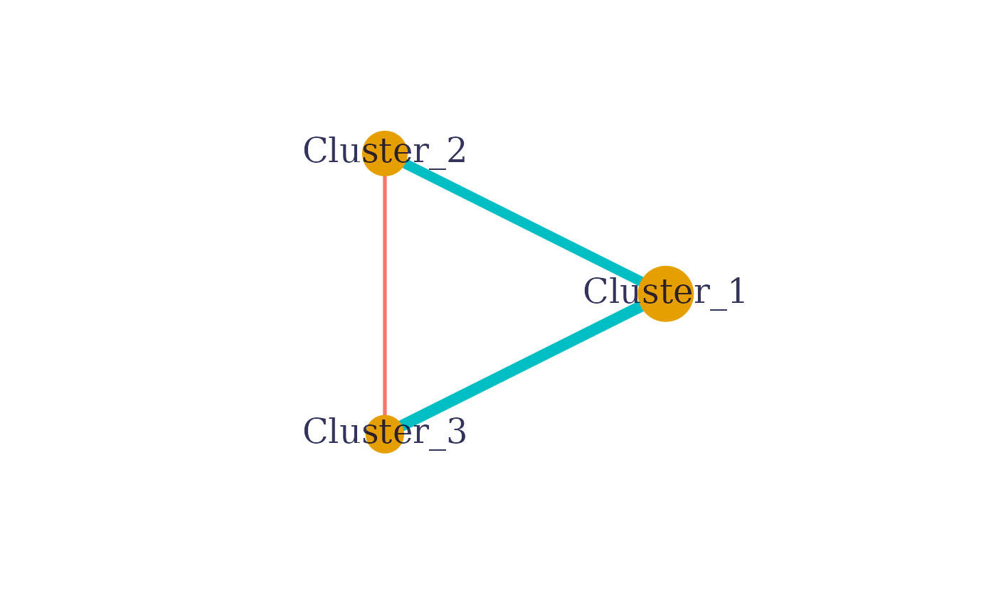
Fixed number of clusters
When the variables’ clustering is unknown, the number of clusters can
simply be fixed via the blocks argument.
my_NB <- normal_block(data = my_data,
blocks = 3)
#> Fitting a diagonal normal-block-var model with 3 unknown blocks
#>
#> DONE
print(my_NB)
#> A diagonal normal-block-var model with 3 unknown blocks .
#> ===========================================================================
#> nb_param q n_edges sparsity loglik deviance BIC ICL EBIC
#> 128 3 3 0 -1678.676 3357.351 3946.813 3294.689 3953.405
#> niter
#> 7
#> ===========================================================================
#> * Useful fields
#> $model_par, $posterior_par / $var_par, $clustering
#> $loglik, $BIC, $ICL, $objective, $nb_param, $criteria
#> * Useful S3 methods
#> print(), summary(), plot(), coef(), sigma(), fitted(), predict()
plot(my_NB)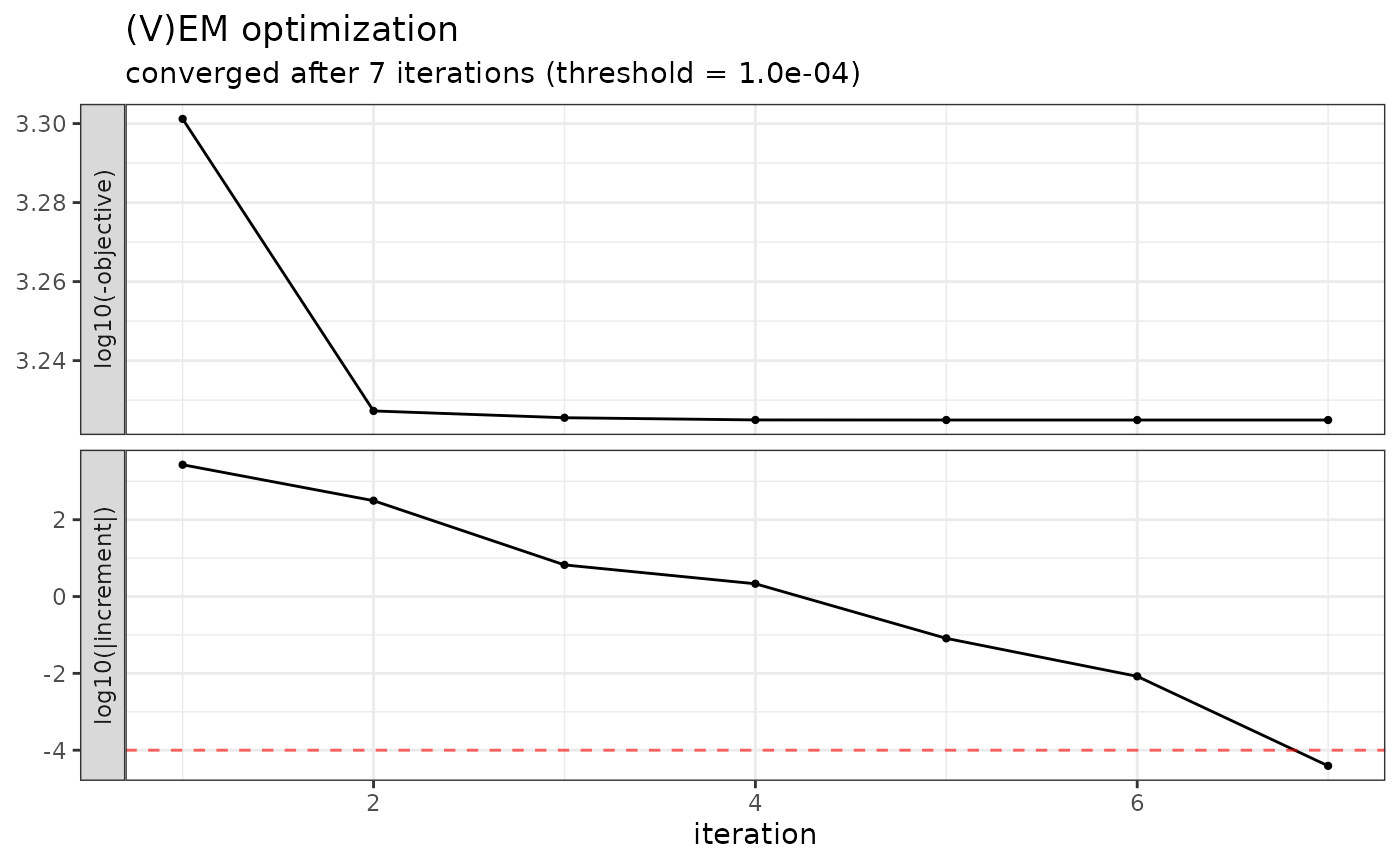 The clustering inferred by
 normal_block() can be compared
with the true clustering, when it is known:
Unknown number of clusters
When the number of clusters is unknown, normal_block()
can be given a range of candidate values instead, returning a collection
of Normal-Block models, one per number of clusters.
my_NB_unknown <- normal_block(data = my_data,
                              blocks = 2:5)
#> Fitting a diagonal normal-block-var model with unknown q
#>   number of blocks = 2                number of blocks = 3                number of blocks = 4                number of blocks = 5
#> DONE
my_NB_unknown is a collection of Normal-Block models. A
specific one can be selected either by its number of clusters or as the
best model for a given criterion (BIC, deviance, EBIC or ICL). The value
of each criterion, for every model in the collection, can be visualized
with plot().
plot(my_NB_unknown)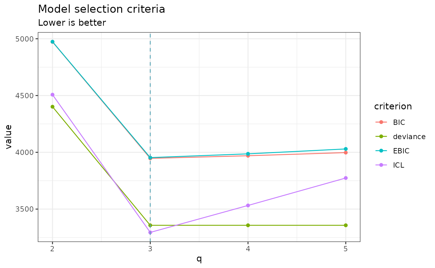
Model selection is done with get_model() when a specific
number of clusters is required, and with get_best_model()
to select the best model for a given criterion.
myNB_3   <- my_NB_unknown$get_model(3)
myNB_BIC <- my_NB_unknown$get_best_model("BIC")
Playing with sparsity
By default, no penalty is applied to the association network. A
penalty can be added via the sparsity argument of
normal_block(), with any of the parametrizations seen above
(fixed clustering, fixed number of clusters, or unknown number of
clusters). The example below uses a fixed clustering.
To use a fixed
penalty (Tous and Chiquet 2026) on the
network, pass that value to the sparsity argument:
my_NB_sparse_low <- normal_block(data = my_data,
                                 blocks = my_nb_data$parameters$C,
                                 sparsity = 0.1)
#> Fitting a diagonal normal-block-var model with fixed blocks
#>
#> DONE
my_NB_sparse_high <- normal_block(data = my_data,
                                  blocks = my_nb_data$parameters$C,
                                  sparsity = 10)
#> Fitting a diagonal normal-block-var model with fixed blocks
#>
#> DONE
The larger the penalty, the sparser the network.
my_NB_sparse_low$plot_network()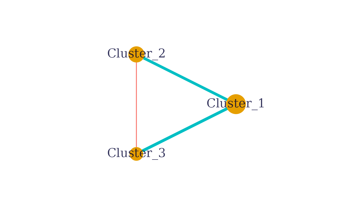
my_NB_sparse_high$plot_network()
#> Warning: vertex attribute label.cex contains NAs. Replacing with default
#> value 1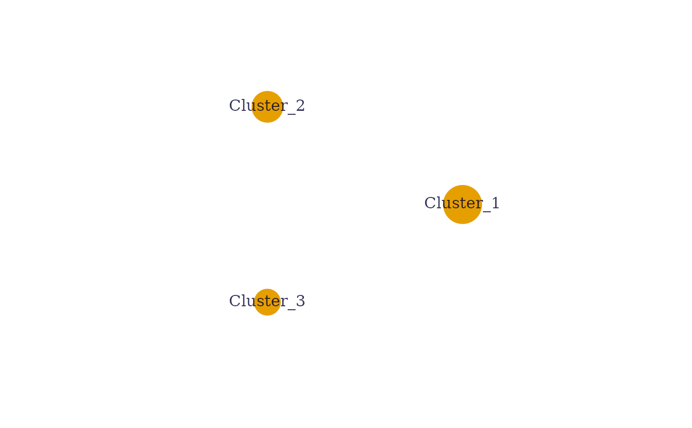 It is usually hard to know a priori which sparsity penalty is best.
normal_block() can instead explore a range of sparsity
levels by simply setting sparsity = TRUE, which returns a
collection of Normal-Block models, one per sparsity penalty.
my_NB_sparse <- normal_block(data = my_data,
                             blocks = my_nb_data$parameters$C,
                             sparsity = TRUE)
#> Fitting a Collection of diagonal normal-block-var models with fixed blocks, with different sparsity penalties.
#>   penalty = 0.3003413             penalty = 0.2562416             penalty = 0.2186171             penalty = 0.1865171             penalty = 0.1591304             penalty = 0.1357649             penalty = 0.1158303             penalty = 0.09882265                penalty = 0.08431231                penalty = 0.07193255                penalty = 0.06137054                penalty = 0.05235937                penalty = 0.04467133                penalty = 0.03811214                penalty = 0.03251606                penalty = 0.02774165                penalty = 0.02366829                penalty = 0.02019302                penalty = 0.01722804                penalty = 0.01469841                penalty = 0.01254021                penalty = 0.0106989             penalty = 0.00912796                penalty = 0.007787682               penalty = 0.0066442             penalty = 0.005668618               penalty = 0.004836282               penalty = 0.004126161               penalty = 0.003520308               penalty = 0.003003413
#> DONE
The different criteria can then be plotted as a function of the
penalty, using plot().
plot(my_NB_sparse)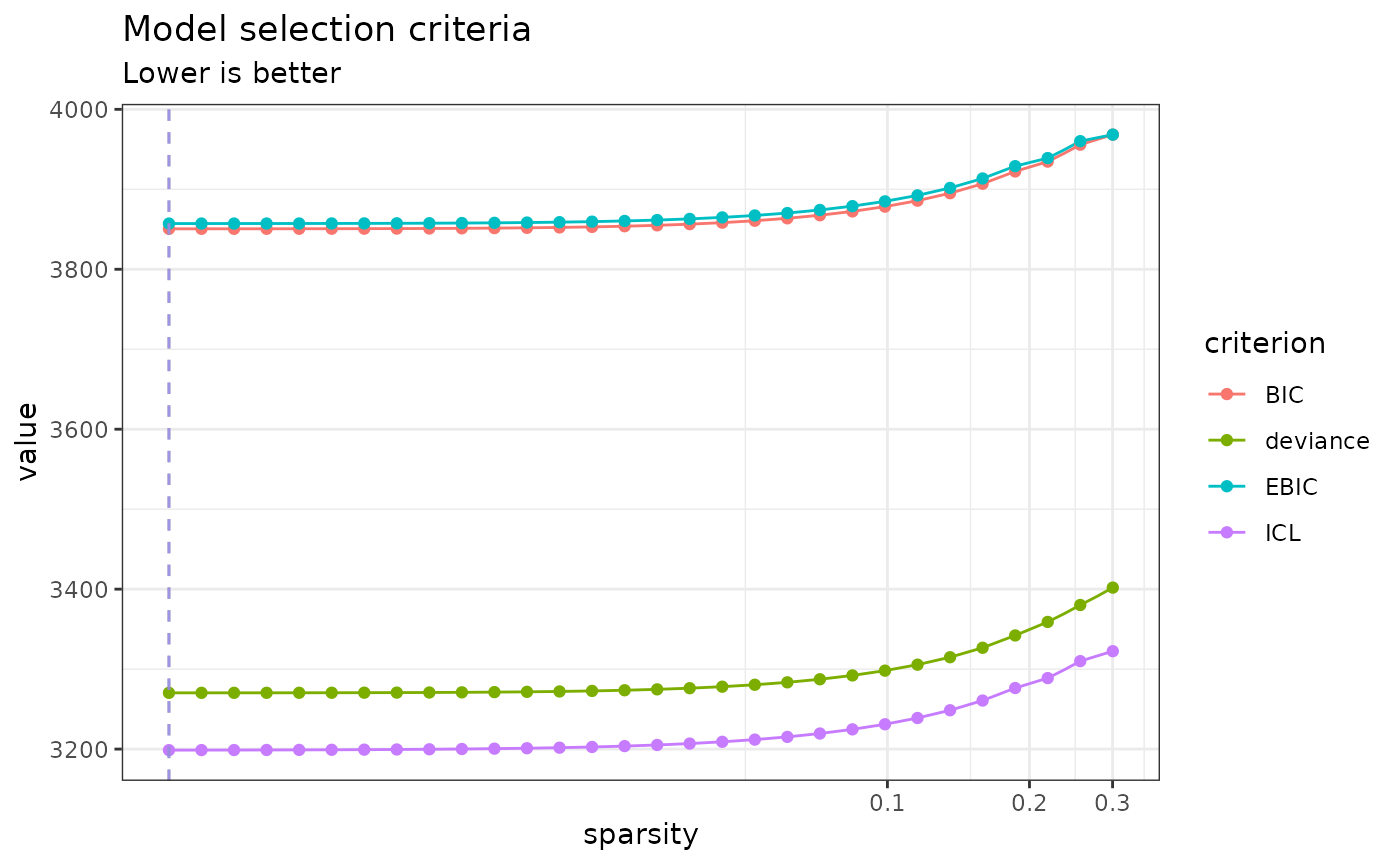 Penalty selection can be done similarly to the selection of the number
of clusters.
Penalty selection can be done similarly to the selection of the number
of clusters.
myNB_sparse_0.1   <- my_NB_sparse$get_model(0.1)
#> No model with this penalty in the collection. Returning model with closest penalty: 0.0988226469658165 Collection penalty values can be found via $sparsity
myNB_sparse_BIC   <- my_NB_sparse$get_best_model("BIC")
Both the sparsity penalty and the number of clusters can also be left to vary jointly.
my_NB_sparse_unknown <-  normal_block(data = my_data,
                                      blocks = 2:6,
                                      sparsity = TRUE)
#> Fitting a Collection of diagonal normal-block-var models with different values of q and different penalties.
#>   number of blocks = 2                penalty = 0.300901              penalty = 0.256719              penalty = 0.2190244             penalty = 0.1868646             penalty = 0.1594269             penalty = 0.1360179             penalty = 0.1160461             penalty = 0.09900679                penalty = 0.08446941                penalty = 0.07206659                penalty = 0.0614849             penalty = 0.05245694                penalty = 0.04475457                penalty = 0.03818316                penalty = 0.03257665                penalty = 0.02779335                penalty = 0.02371239                penalty = 0.02023065                penalty = 0.01726014                penalty = 0.0147258             penalty = 0.01256358                penalty = 0.01071884                penalty = 0.009144969               penalty = 0.007802193               penalty = 0.006656581               penalty = 0.005679181               penalty = 0.004845294               penalty = 0.004133849               penalty = 0.003526867               penalty = 0.00300901                number of blocks = 3                penalty = 0.3002468             penalty = 0.2561609             penalty = 0.2185482             penalty = 0.1864583             penalty = 0.1590802             penalty = 0.1357222             penalty = 0.1157938             penalty = 0.09879153                penalty = 0.08428576                penalty = 0.0719099             penalty = 0.06135121                penalty = 0.05234288                penalty = 0.04465727                penalty = 0.03810014                penalty = 0.03250582                penalty = 0.02773292                penalty = 0.02366083                penalty = 0.02018666                penalty = 0.01722261                penalty = 0.01469378                penalty = 0.01253626                penalty = 0.01069553                penalty = 0.009125086               penalty = 0.00778523                penalty = 0.006642108               penalty = 0.005666833               penalty = 0.00483476                penalty = 0.004124861               penalty = 0.003519199               penalty = 0.003002468               number of blocks = 4                penalty = 0.4133606             penalty = 0.3526659             penalty = 0.3008832             penalty = 0.2567039             penalty = 0.2190115             penalty = 0.1868536             penalty = 0.1594175             penalty = 0.1360099             penalty = 0.1160392             penalty = 0.09900095                penalty = 0.08446443                penalty = 0.07206234                penalty = 0.06148127                penalty = 0.05245384                penalty = 0.04475193                penalty = 0.03818091                penalty = 0.03257472                penalty = 0.02779171                penalty = 0.02371099                penalty = 0.02022946                penalty = 0.01725912                penalty = 0.01472493                penalty = 0.01256283                penalty = 0.01071821                penalty = 0.009144429               penalty = 0.007801733               penalty = 0.006656188               penalty = 0.005678846               penalty = 0.004845009               penalty = 0.004133606               number of blocks = 5                penalty = 0.4229238             penalty = 0.360825              penalty = 0.3078443             penalty = 0.2626428             penalty = 0.2240784             penalty = 0.1911765             penalty = 0.1631056             penalty = 0.1391565             penalty = 0.1187238             penalty = 0.1012914             penalty = 0.08641854                penalty = 0.07372952                penalty = 0.06290366                penalty = 0.05366738                penalty = 0.04578728                penalty = 0.03906424                penalty = 0.03332835                penalty = 0.02843468                penalty = 0.02425955                penalty = 0.02069747                penalty = 0.01765842                penalty = 0.01506559                penalty = 0.01285348                penalty = 0.01096618                penalty = 0.009355989               penalty = 0.007982229               penalty = 0.006810181               penalty = 0.005810227               penalty = 0.004957099               penalty = 0.004229238               number of blocks = 6                penalty = 0.42662               penalty = 0.3639785             penalty = 0.3105348             penalty = 0.2649383             penalty = 0.2260368             penalty = 0.1928473             penalty = 0.1645312             penalty = 0.1403727             penalty = 0.1197615             penalty = 0.1021766             penalty = 0.08717382                penalty = 0.0743739             penalty = 0.06345342                penalty = 0.05413642                penalty = 0.04618745                penalty = 0.03940565                penalty = 0.03361963                penalty = 0.02868319                penalty = 0.02447158                penalty = 0.02087836                penalty = 0.01781275                penalty = 0.01519726                penalty = 0.01296582                penalty = 0.01106202                penalty = 0.009437758               penalty = 0.008051992               penalty = 0.0068697             penalty = 0.005861007               penalty = 0.005000423               penalty = 0.0042662
#> DONE
The result is a collection of Normal-Block models with different numbers of clusters and different penalties.
my_NB_sparse_unknown$who_am_I
#> [1] "Collection of diagonal normal-block-var models with different values of q and different penalties."
plot() allows each criterion to be analysed as a
function of both the number of clusters and the penalty. By default, the
penalties tested are computed by normal_block() separately
for each number of clusters, and can differ from one to another – which
is what the blanks in the plot come from.
plot(my_NB_sparse_unknown, "BIC")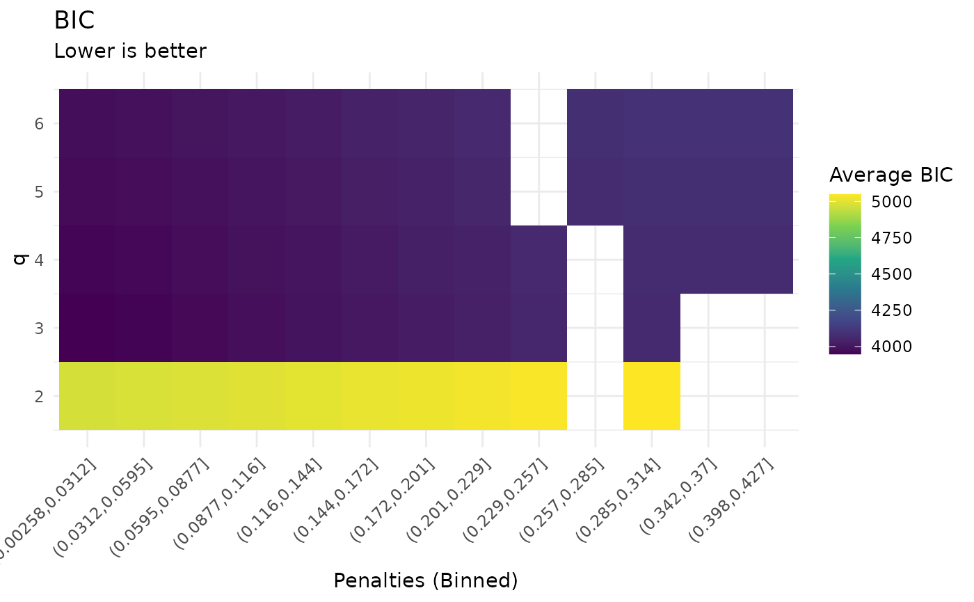
Model selection is also done using get_model() and
get_best_model(). With get_model(), one can
fix only the number of clusters, getting back a collection of models
with different sparsity levels, or fix both the number of clusters and
the sparsity level.
my_NB_sparse_3     <- my_NB_sparse_unknown$get_model(3)
my_NB_sparse_3_0.1 <- my_NB_sparse_unknown$get_model(3, 0.1)
#> No model with this penalty in the collection. Returning model with closest penalty: 0.0987915298048486 Collection penalty values can be found via $sparsity
With zero-inflated data
The process is similar with zero-inflated data, but
zero_inflation = TRUE must be passed to
normal_block(). The example below uses a fixed number of
blocks and no penalty on the network.
my_NB_zi <- normal_block(data = my_data_zi,
                         blocks = 4,
                         zero_inflation = TRUE)
#> Fitting a zero-inflated diagonal normal-block-var model with 4 unknown blocks
#>
#> DONE
When the data is zero-inflated, the inference process may take longer.
plot(my_NB_zi)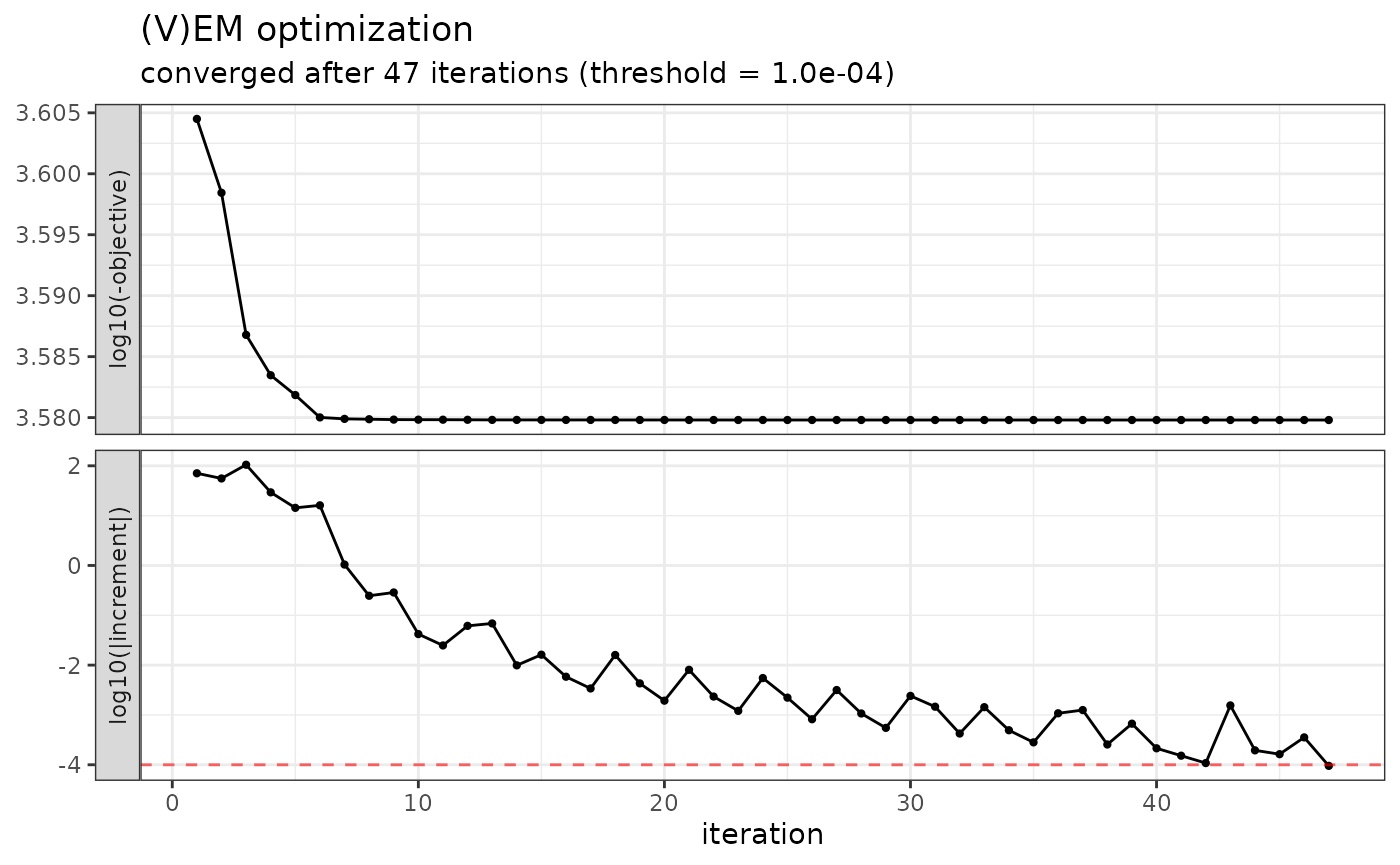
The clustering inference may also be harder.