Gaussian Graphical Models with Latent Clustering Structure • normalblockr

Description

The Normal-Block model¹ is a Gaussian graphical model with a latent clustering structure, designed for the multivariate analysis of continuous data: it clusters variables and, building on the graphical lasso, infers a network of statistical dependencies between clusters rather than between individual variables. This package implements an efficient (variational) EM algorithm to fit it, accompanied by a set of functions for model selection, visualization and diagnostic. See all the dedicated vignettes for a comprehensive introduction.

normalblockr covers the following model variants, all built around the same normal_block()/NormalBlockData interface:

Known clusters: the grouping of variables is given (e.g. from prior knowledge); only the association network between clusters is estimated, by EM.
Unknown clusters: the grouping is inferred jointly with everything else by a variational EM, either for a single number of clusters or over a range explored as a collection, with model selection via BIC/EBIC/ICL.
Sparse (graphical-lasso) network: an $\ell_1$ penalty² on the inter-cluster precision matrix, for a single penalty value or a path explored as a collection.
Zero-inflated extension: an excess-of-zeros layer for data (e.g. abundance/biomass tables) with more exact zeros than a plain Normal model can represent.

Any combination of these is reached through the same normal_block() function: known or unknown clustering, sparse or not, zero-inflated or not are independent choices, not separate model classes to learn.

Since version 0.3.0 the package also fits a second, complementary family, reached with normal_block(..., model = "mean"):

Mean-block models: variables are clustered by how they respond to the covariates rather than by how they covary. All variables in a cluster share one regression profile, so the mean is $\mu_i = C B^\top X_i$ with $B$ of size $d \times q$ instead of $d \times p$ . Known or unknown clustering, zero-inflated or not, with the residual covariance taken diagonal (the default), spherical, or full.

The two families answer different questions and generally return different groupings; normal_block_sequential() runs one after the other when both are of interest. See the mean-block vignette.

Installation

Install the released version from CRAN:

install.packages("normalblockr")

or the development version from GitHub:

# install.packages("pak")
pak::pak("jchiquet/normalblockr")

Illustration

We illustrate the known-/unknown-clusters and sparse variants on brca_rppa³: reverse-phase protein array measurements of 163 proteins across 346 breast cancer tumor samples from The Cancer Genome Atlas, together with each sample’s PAM50 molecular subtype.

library(normalblockr)
data(brca_rppa)
Y    <- as.matrix(brca_rppa$expr)
X    <- model.matrix(~ 0 + PAM50_SUBTYPE, data = brca_rppa$covariates)
data <- NormalBlockData$new(Y, X)

Known clusters

A simple, fully data-driven grouping (hierarchical clustering on the raw expression profiles, with no reference to the Normal-Block model) handed to normal_block() as fixed – only the network between the 6 blocks is estimated.

hc    <- brca_rppa$expr |> scale() |> t() |> dist() |> hclust("ward.D2")
group <- cutree(hc, 6) |> normalblockr:::as_indicator()
m_known <- normal_block(data, blocks = group)

Fitting a diagonal normal-block-var model with fixed blocks 

DONE

m_known

A diagonal normal-block-var model with fixed blocks .
===========================================================================
 nb_param q n_edges sparsity    loglik deviance      BIC      ICL   EBIC niter
      999 6      15        0 -70387.84 140775.7 146616.3 144073.3 146670    14
===========================================================================
* Useful fields
    $model_par, $posterior_par / $var_par, $clustering 
    $loglik, $BIC, $ICL, $objective, $nb_param, $criteria
* Useful S3 methods
    print(), summary(), plot(), coef(), sigma(), fitted(), predict()

Unknown number of clusters

Leave the clustering for the model to infer, over a range of candidate cluster counts explored as a collection, then select by ICL.

m_unknown <- normal_block(data, blocks = 2:20)

Fitting a diagonal normal-block-var model with unknown q 
     number of blocks = 2           
     number of blocks = 3           
     number of blocks = 4           
     number of blocks = 5           
     number of blocks = 6           
     number of blocks = 7           
     number of blocks = 8           
     number of blocks = 9           
     number of blocks = 10           
     number of blocks = 11           
     number of blocks = 12           
     number of blocks = 13           
     number of blocks = 14           
     number of blocks = 15           
     number of blocks = 16           
     number of blocks = 17           
     number of blocks = 18           
     number of blocks = 19           
     number of blocks = 20           
DONE

m_unknown$refine(verbose = FALSE)
m_unknown$plot(c("deviance", "BIC", "ICL", "EBIC"))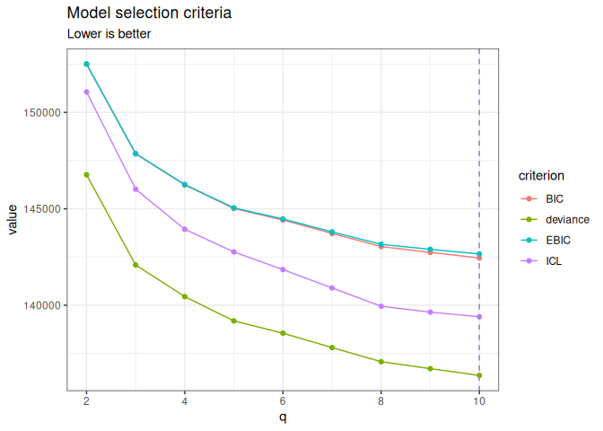

m_unknown$get_best_model("EBIC")

A diagonal normal-block-var model with 16 unknown blocks .
===========================================================================
 nb_param  q n_edges sparsity    loglik deviance      BIC      ICL     EBIC
     1129 16     120        0 -67374.79 134749.6 141350.2 137746.6 142015.6
 niter
    32
===========================================================================
* Useful fields
    $model_par, $posterior_par / $var_par, $clustering 
    $loglik, $BIC, $ICL, $objective, $nb_param, $criteria
* Useful S3 methods
    print(), summary(), plot(), coef(), sigma(), fitted(), predict()

Sparse network

Treating a clustering as fixed (known, or selected above), explore a path of graphical-lasso penalties on the inter-cluster network and select by BIC. Unlike the dense, unpenalized network, this is the one actually worth visualizing.

m_sparse <- normal_block(data, blocks = group, sparsity = TRUE)

Fitting a Collection of diagonal normal-block-var models with fixed blocks, with different sparsity penalties. 
     penalty = 0.2565018           
     penalty = 0.2188391           
     penalty = 0.1867065           
     penalty = 0.1592919           
     penalty = 0.1359028           
     penalty = 0.1159479           
     penalty = 0.098923           
     penalty = 0.08439792           
     penalty = 0.07200559           
     penalty = 0.06143286           
     penalty = 0.05241254           
     penalty = 0.04471669           
     penalty = 0.03815085           
     penalty = 0.03254907           
     penalty = 0.02776982           
     penalty = 0.02369232           
     penalty = 0.02021353           
     penalty = 0.01724553           
     penalty = 0.01471333           
     penalty = 0.01255294           
     penalty = 0.01070977           
     penalty = 0.009137229           
     penalty = 0.00779559           
     penalty = 0.006650947           
     penalty = 0.005674374           
     penalty = 0.004841193           
     penalty = 0.004130351           
     penalty = 0.003523882           
     penalty = 0.003006463           
     penalty = 0.002565018           
DONE

sp_best  <- m_sparse$get_best_model("BIC")
sp_best$plot_network()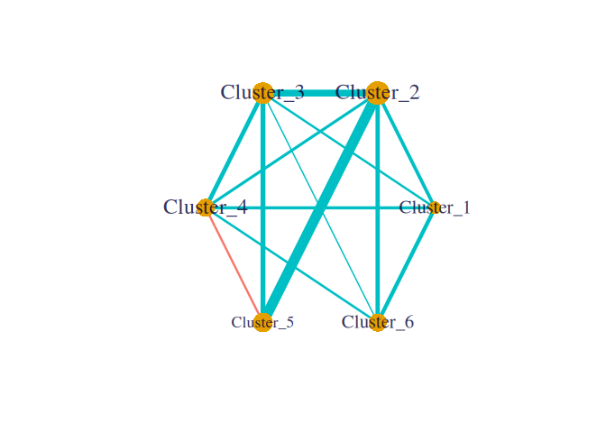

Zero-inflated data

For data with an excess of exact zeros beyond what a plain Normal model would represent (e.g. abundance/biomass tables), zero_inflation = TRUE adds a per-variable excess-of-zero layer. Illustrated on onema⁴: total biomass of 46 fish species across 399 French stream electrofishing stations, where seven in ten entries are exact zeros.

data(onema)
X_zi    <- model.matrix(~ 1 + temperature_med, data = onema$covariates)
Y_zi    <- log(1 + onema$biomass)
data_zi <- NormalBlockData$new(Y_zi, X_zi)
m_zi    <- normal_block(data_zi, blocks = 2:8, zero_inflation = TRUE)

Fitting a diagonal normal-block-var model with unknown q 
     number of blocks = 2           
     number of blocks = 3           
     number of blocks = 4           
     number of blocks = 5           
     number of blocks = 6           
     number of blocks = 7           
     number of blocks = 8           
DONE

m_zi$get_best_model("ICL")

A zero-inflated diagonal normal-block-var model with 6 unknown blocks .
===========================================================================
 nb_param q n_edges sparsity    loglik deviance      BIC      ICL     EBIC
      210 6      15        0 -13519.35 27038.71 28296.39 27090.47 28350.14
 niter
    20
===========================================================================
* Useful fields
    $model_par, $posterior_par / $var_par, $clustering 
    $loglik, $BIC, $ICL, $objective, $nb_param, $criteria
* Useful S3 methods
    print(), summary(), plot(), coef(), sigma(), fitted(), predict()

Learning more

normal-block (vignette("normal-block")): a general introduction on simulated data – known/unknown clusters, sparsity, zero-inflation.
zero-inflated-normal-block (vignette("zero-inflated-normal-block")): a full worked example on onema, with the math behind the zero-inflation extension.
breast-cancer-proteomics (vignette("breast-cancer-proteomics")): a full worked example on brca_rppa – known vs. inferred clustering, model selection, the post-hoc refine() step, sparsifying the selected network.
mean-block-breast-cancer (vignette("mean-block-breast-cancer")): the mean-block family on brca_rppa – clustering proteins by their subtype signature, choosing the shape of the residual covariance, sparsifying it.
inst/normal_block_models.qmd in the package sources: a reference card in two parts, the models (both families, with their criteria and E/M or VE/M updates) and the implementation notes.

Note on the use of generative AI

The models implemented here – their definition and every algebraic derivation – were worked out by Jeanne Tous and Nestor Ngalala Manguitini and their advisor, Julien Chiquet, over a PhD thesis and a Master’s research internship respectively, who also wrote the first working versions of the code, its object-oriented architecture, and the first simulation studies. Generative AI (Claude Sonnet and Claude Opus, Anthropic) was used afterwards to improve the documentation, produce synthesis material, and audit, test and improve the code – in particular to port several algorithmic components to C++, including the graphical lasso solver, whose original R-callback implementation caused intermittent memory crashes. See the technical report for details.

normalblockr: Gaussian graphical models with latent clustering structure for multivariate continuous data