library(tidyverse)
library(gridExtra)
library(GGally)
library(mclust)
library(aricode)
library(VGAM)
library(palmerpenguins)
theme_set(theme_bw())Clustering and classification with model based approaches
An short example study on the penguins dataset
Preliminary
Functions from R-base and stats (preloaded) are required plus packages from the tidyverse for data representation and manipulation. We also need the package mclust, which are commonly used to fit mixture models in R, as weel as palmerpenguins for the illustrative data set. aricode is used for clustering comparison, VGAM to fit multinomial models.
1 The Palmer penguins data set
The palmerpenguins data 1 (Horst, Hill, and Gorman (2020)) contains size measurements for three penguin species observed on three islands in the Palmer Archipelago, Antarctica.
These data were collected from 2007 - 2009 by Dr. Kristen Gorman with the Palmer Station Long Term Ecological Research Program, part of the US Long Term Ecological Research Network. The data were imported directly from the Environmental Data Initiative (EDI) Data Portal, and are available for use by CC0 license (“No Rights Reserved”) in accordance with the Palmer Station Data Policy.
This data et is an alternative to Anderson’s Iris data (see datasets::iris). There are both a nice example for learning supervised classification algorithms, and is known as a difficult case for unsupervised learning.
data("penguins", package = "palmerpenguins")
penguins %>% rmarkdown::paged_table()
We remove row with NA values and columns year, island and sex to only keep the four continuous attributes and the species of each individual:
penguins <- penguins %>% drop_na() %>%
  select(-year, -island, -sex)
The pair plot show some structure that could find by clustering or descreibe by a Gaussian mixture model:
species_col <- c("darkorange","purple","cyan4")
ggpairs(penguins, columns = c(2:5), aes(color = species)) +
    scale_color_manual(values = species_col) +
    scale_fill_manual(values = species_col)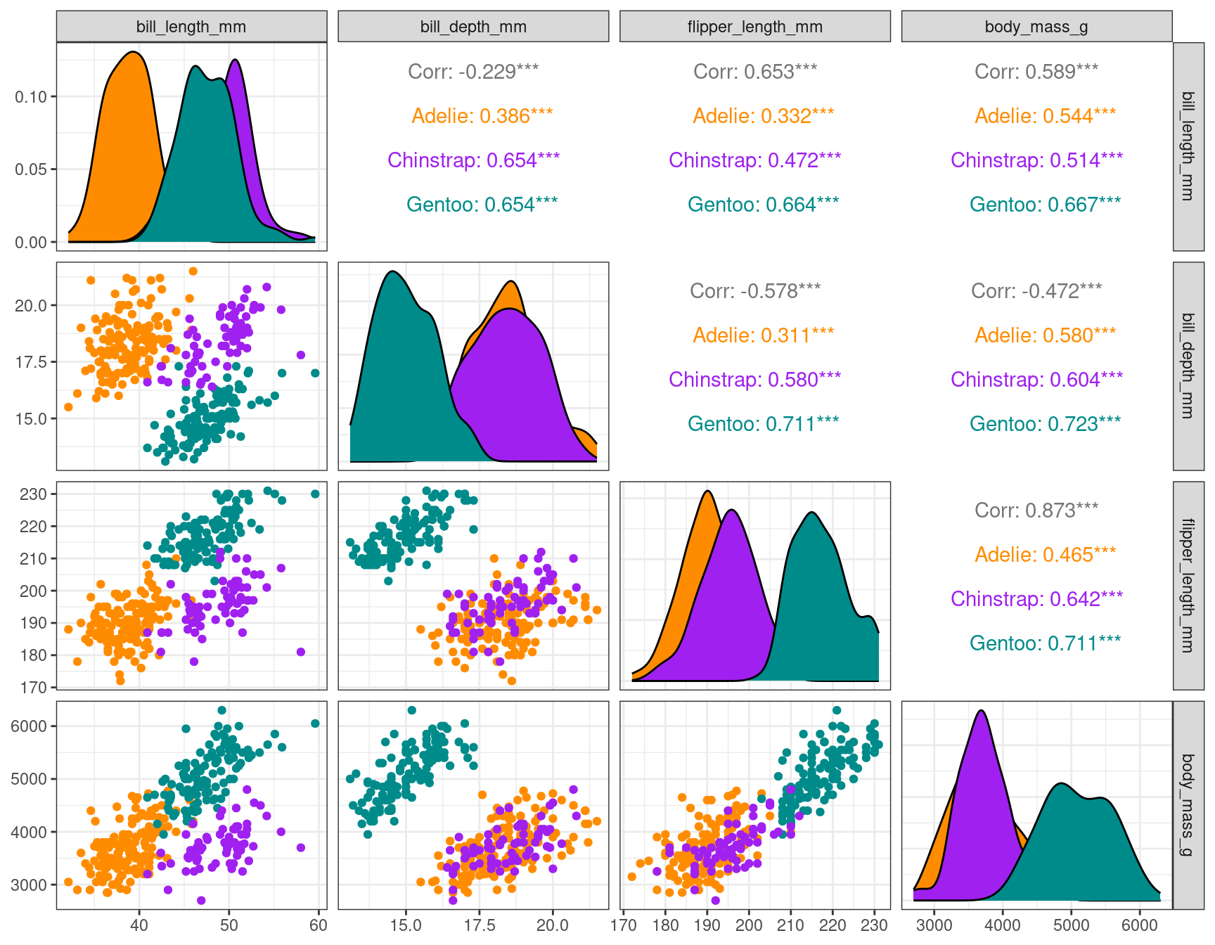
1.1 Supervised classification
1.1.1 Logistic regression for a binary variable
Let y_i be a binary response that take its values in \{0,1\} and let c_{i1}, \ldots, c_{iM} be M explanatory variables (or predictors).
Formally, the logistic regression model is that
\log\left(\frac{\mathbb{P}(y_i=1)}{\mathbb{P}(y_i=0)}\right) = \log\left(\frac{\mathbb{P}(y_i=1)}{1 - \mathbb{P}(y_i=1)}\right) = \beta_0 + \sum_{m=1}^M \beta_m c_{im} Then,
\mathbb{P}(y_i=1) = \frac{1}{1+ e^{-\beta_0 - \sum_{m=1}^M \beta_m c_{im}}}
We try to predict the binary indicator variable for species Adelie with this model:
penguins <- penguins %>% mutate(adelie = (species == 'Adelie') * 1)
logistic_Adelie <- glm(
  adelie ~
    bill_length_mm +
    bill_depth_mm  +
    flipper_length_mm +
    body_mass_g, family = binomial, data = penguins)
summary(logistic_Adelie)
Call:
glm(formula = adelie ~ bill_length_mm + bill_depth_mm + flipper_length_mm +
    body_mass_g, family = binomial, data = penguins)

Deviance Residuals:
   Min      1Q  Median      3Q     Max
-1.328   0.000   0.000   0.000   1.652

Coefficients:
                   Estimate Std. Error z value Pr(>|z|)
(Intercept)       27.195927  28.156975   0.966   0.3341
bill_length_mm    -5.106876   2.730998  -1.870   0.0615 .
bill_depth_mm      8.953805   5.014702   1.786   0.0742 .
flipper_length_mm  0.052471   0.119287   0.440   0.6600
body_mass_g        0.006281   0.003952   1.589   0.1120
---
Signif. codes:  0 '***' 0.001 '**' 0.01 '*' 0.05 '.' 0.1 ' ' 1

(Dispersion parameter for binomial family taken to be 1)

    Null deviance: 456.5751  on 332  degrees of freedom
Residual deviance:   9.4492  on 328  degrees of freedom
AIC: 19.449

Number of Fisher Scoring iterations: 13
The linear predictor can be recovered as follows (e.g. for penguins #127)
X <- as.matrix(cbind(1, penguins[, 2:5]))
beta <- coefficients(logistic_Adelie)
all.equal(
  predict(logistic_Adelie, type = "link"),
  as.numeric(X %*% beta),
  check.attributes = FALSE)
[1] TRUEThe fitted value as follows:
all.equal(
  predict(logistic_Adelie, type = "response"),
  as.numeric(1 / ( 1 + exp( - (X %*% beta)))),
 check.attributes = FALSE)
[1] TRUEThe ARI is close to 1 in that case
aricode::ARI(penguins$adelie, round(predict(logistic_Adelie, type = "response")))[1] 0.96417511.1.2 Logistic regression with more than two classes
Assume now that y_i takes its values in \{1,2\ldots,L\}. The logistic regression model now writes
\log\left(\frac{\mathbb{P}(y_i=k)}{\mathbb{P}(y_i=L)}\right) = \beta_{k0} + \sum_{m=1}^M \beta_{k m} c_{im} \quad , \quad k=1,2,\ldots,L where we set, for instance, \beta_{L0}=\beta_{L1}=\ldots=\beta_{LM}=0 for identifiabilty reason. Then,
\mathbb{P}(y_i=k) = \frac{e^{\beta_{k0} + \sum_{m=1}^M \beta_{k m} c_{im}}} {\sum_{j=1}^K e^{\beta_{j0} + \sum_{m=1}^M \beta_{j m} c_{im}}} \quad , \quad k=1,2,\ldots,L Let us first code all species modalities as dummy variables:
penguins <- penguins %>%
  mutate(gentoo    = (species == 'Gentoo') * 1) %>%
  mutate(chinstrap = (species == 'Chinstrap') * 1)
penguins %>% rmarkdown::paged_table()
We now fit a multinomial model to this 3-class problem:
multinomial_penguins <-
  vglm(cbind(gentoo, adelie, chinstrap) ~
    bill_length_mm +
    bill_depth_mm  +
    flipper_length_mm +
    body_mass_g, family = multinomial, data = penguins)
summary(multinomial_penguins)
Call:
vglm(formula = cbind(gentoo, adelie, chinstrap) ~ bill_length_mm +
    bill_depth_mm + flipper_length_mm + body_mass_g, family = multinomial,
    data = penguins)

Coefficients:
                     Estimate Std. Error z value Pr(>|z|)
(Intercept):1        7.294722  60.956154   0.120  0.90474
(Intercept):2       26.107462  22.696081   1.150  0.25002
bill_length_mm:1    -1.298442   1.061332  -1.223  0.22118
bill_length_mm:2    -3.207140   1.205017  -2.661  0.00778 **
bill_depth_mm:1     -1.532394   1.462216  -1.048  0.29464
bill_depth_mm:2      3.341561   1.951686      NA       NA
flipper_length_mm:1  0.170417   0.316373   0.539  0.59012
flipper_length_mm:2  0.095995   0.125187      NA       NA
body_mass_g:1        0.010319   0.006946   1.486  0.13739
body_mass_g:2        0.009378   0.004705   1.993  0.04624 *
---
Signif. codes:  0 '***' 0.001 '**' 0.01 '*' 0.05 '.' 0.1 ' ' 1

Names of linear predictors: log(mu[,1]/mu[,3]), log(mu[,2]/mu[,3])

Residual deviance: 5.7536 on 656 degrees of freedom

Log-likelihood: -2.8768 on 656 degrees of freedom

Number of Fisher scoring iterations: 18

Warning: Hauck-Donner effect detected in the following estimate(s):
'bill_depth_mm:2', 'flipper_length_mm:2'


Reference group is level  3  of the response
posterior_prob <- predict(multinomial_penguins, type = "response")Warning in object@family@linkinv(eta = object@predictors, extra = new.extra):
fitted probabilities numerically 0 or 1 occurredmatplot(posterior_prob)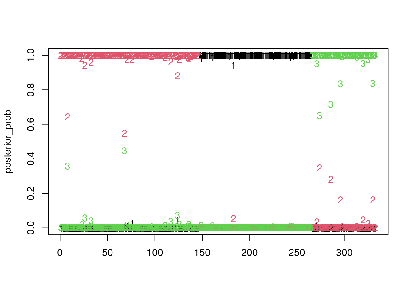
clustering_map <- apply(posterior_prob, 1, which.max)we get a perfect clustering of the penguins with this model (on the training set!)
clustering_map <- apply(posterior_prob, 1, which.max)
aricode::ARI(clustering_map, penguins$species)
[1] 11.2 Non supervised classification
Ignoring the known labels (species) of the penguin data, let us identify three clusters with the k-means method and compute the missclassification rate:
kclust <- kmeans(penguins[, 2:5], centers = 3, nstart = 10)
aricode::ARI(kclust$cl,  penguins$species)
[1] 0.3212539Let us know fit a mixture of three multidimensional Gaussian distributions.
Function Mclust fits many multivariate Gaussian mixture model, with various parametric form for the covariances. Let us force the model to have spherical variance with equal volume (thus close to the k-means setting):
GMM_EII <- Mclust(penguins[, 2:4], G = 3, modelNames = 'EII')The fit is poor
plot(GMM_EII, "classification")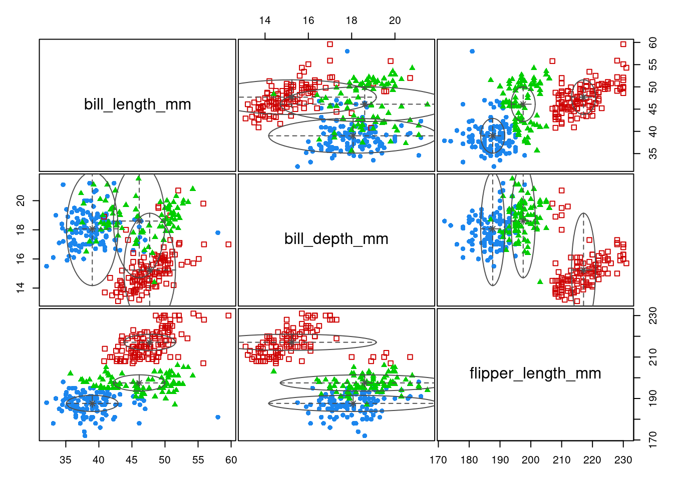
aricode::ARI(penguins$species, map(GMM_EII$z))[1] 0.6363721We can let Mclust chose the “best” model, relying on BIC: we found “VVE”, an ellipsoidal model with equal orientation
GMM_best <- Mclust(penguins[, 2:4], G = 3)
plot(GMM_best, "classification")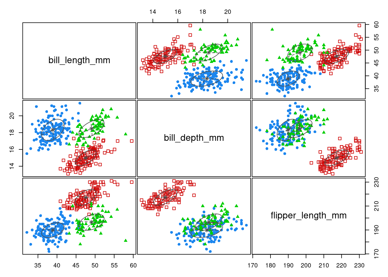
summary(GMM_best, parameters = TRUE)----------------------------------------------------
Gaussian finite mixture model fitted by EM algorithm
----------------------------------------------------
Mclust VVE (ellipsoidal, equal orientation) model with 3 components:
log-likelihood n df BIC ICL
-2647.114 333 23 -5427.815 -5441.159
Clustering table:
1 2 3
150 119 64
Mixing probabilities:
1 2 3
0.4468457 0.3573179 0.1958364
Means:
[,1] [,2] [,3]
bill_length_mm 38.91639 47.56843 49.05177
bill_depth_mm 18.32181 14.99638 18.48159
flipper_length_mm 189.90109 217.23500 196.53408
Variances:
[,,1]
bill_length_mm bill_depth_mm flipper_length_mm
bill_length_mm 8.744628 1.529139 7.411096
bill_depth_mm 1.529139 1.622307 3.249674
flipper_length_mm 7.411096 3.249674 38.620270
[,,2]
bill_length_mm bill_depth_mm flipper_length_mm
bill_length_mm 7.470233 1.5733271 9.389060
bill_depth_mm 1.573327 0.8783978 3.965065
flipper_length_mm 9.389060 3.9650651 45.191222
[,,3]
bill_length_mm bill_depth_mm flipper_length_mm
bill_length_mm 11.020717 2.043209 9.017857
bill_depth_mm 2.043209 1.134670 4.030423
flipper_length_mm 9.017857 4.030423 47.437865We get an almost perfect clustering with the MAP:
aricode::ARI(penguins$species, map(GMM_best$z))[1] 0.9355119References
Horst, Allison Marie, Alison Presmanes Hill, and Kristen B Gorman. 2020. Palmerpenguins: Palmer Archipelago (Antarctica) Penguin Data. https://doi.org/10.5281/zenodo.3960218.