library(tidyverse)
library(saemix)
library(corrplot)
theme_set(theme_bw())Nonlinear Mixed Effects Models
Exercices
Preliminary
Functions from R-base and stats (preloaded) are required plus packages from the tidyverse for data representation and manipulation. We also need the lme4 package which is the standard for fitting mixed-model. lattice is used for graphical representation of quantities such as random and fixed effects in the mixed models. saemix implements Stochastic EM algorithms to fit non-linear mixed effect models.
1 Introduction
Séralini, Cellier, and Vendomois (2007) published the paper “New Analysis of a Rat Feeding Study with a Genetically Modified Maize Reveals Signs of Hepatorenal Toxicity”. The authors of the paper pretend that, after the consumption of MON863, rats showed slight but dose-related significant variations in growth.
The objective of this exercise is to highlight the flaws in the methodology used to achieve this result, and show how to properly analyse the data.
We will restrict our study to the male rats of the study fed with 11% of maize (control and GMO)
rats <- read_csv("../../data/ratWeight.csv")
males11 <- filter(rats, gender == "Male" & dosage == "11%")
males11 %>% rmarkdown::paged_table()
2 Nonlinear fixed effect model reproducing Seralini et al.’s study
Plot the growth curves of the control and GMO groups.
Fit an Gompertz growth model f_1(t) = A \exp(-\exp(-b(t-c))) to the complete data (males fed with 11% of maize) using a least square approach, with the same parameters for the control and GMO groups.
Fit a Gompertz growth model to the complete data using a least square approach, with different parameters for the control and GMO groups.
Hint: write the model as
y_{ij} = A_{0} e^{-e^{-b_0 (t_{ij}-c_0)}} \mathbf{1}_{\{{\rm regime\}}_i={\rm Control}} + A_{1} e^{- e^{-b_1 (t_{ij}-c_1)}} \mathbf{1}_{\{{\rm regime}_i={\rm GMO}\}} + \varepsilon_{ij}
Check out the results of the paper displayed Table 1, for the 11% males.
Plot the residuals and explain why the results of the paper are wrong.
3 Nonlinear mixed effect model with SAEMIX
We propose to use instead a mixed effects model for testing the effect of the regime on the growth of the 11% male rats.
3.1 Gompertz model with random effects
The codes below show how to fit a Gompertz model to the data
- assuming the same population parameters for the two regime groups,
- using lognormal distributions for the 3 parameters (setting transform.par=c(1,1,1))
- assuming a diagonal covariance matrix \Omega (default)
3.1.1 Data declaration
Create first the saemixData object
saemix_data <- saemixData(
  name.data       = males11,
  name.group      = "id",
  name.predictors = "week",
  name.response   = "weight"
  )
The following SaemixData object was successfully created:

Object of class SaemixData
    longitudinal data for use with the SAEM algorithm
Dataset males11
    Structured data: weight ~ week | id
    Predictor: week ()
3.1.2 Model declaration
Implement then the structural model and create the saemixModel object. Initial values for the population parameters should be provided.
gompertz <- function(psi, id, x) {
  t <- x[,1]
  A <- psi[id, 1]
  b <- psi[id, 2]
  c <- psi[id, 3]
  ypred <- A*exp(-exp(-b*(t-c)))
  ypred
}

psi0 <- c(A = 500, b = 0.2, c = 0.2)
distribParam <- c(1, 1, 1)
NLMM_gompertz <- saemixModel(model = gompertz, psi0 = psi0, transform.par = distribParam)
3.1.3 Model estimation
Run saemix for estimating the population parameters, computing the individual estimates, computing the FIM and the log-likelihood (linearization)
saemix_options <- saemixControl(
  map   = TRUE,
  fim   = TRUE,
  ll.is = FALSE,
  displayProgress = FALSE,
  directory = "output_saemix",
  seed = 12345)
NLMM_gompertz_fit <- saemix(NLMM_gompertz , saemix_data, saemix_options)summary(NLMM_gompertz_fit)----------------------------------------------------
----------------- Fixed effects ------------------
----------------------------------------------------
Parameter Estimate SE CV(%)
1 A 528.150 8.4048 1.59
2 b 0.216 0.0072 3.33
3 c 0.064 0.0799 125.22
4 a.1 12.203 0.4093 3.35
----------------------------------------------------
----------- Variance of random effects -----------
----------------------------------------------------
Parameter Estimate SE CV(%)
A omega2.A 0.0093 0.0022 23.89
b omega2.b 0.0296 0.0096 32.33
c omega2.c 0.1939 0.0560 28.86
----------------------------------------------------
------ Correlation matrix of random effects ------
----------------------------------------------------
omega2.A omega2.b omega2.c
omega2.A 1.00 0.00 0.00
omega2.b 0.00 1.00 0.00
omega2.c 0.00 0.00 1.00
----------------------------------------------------
--------------- Statistical criteria -------------
----------------------------------------------------
Likelihood computed by linearisation
-2LL= 4704.198
AIC = 4718.198
BIC = 4730.02
----------------------------------------------------3.1.4 Diagnostic plots:
# Individual plot for subject 1 to 9,
saemix.plot.fits(NLMM_gompertz_fit, ilist = c(1:9), smooth=TRUE)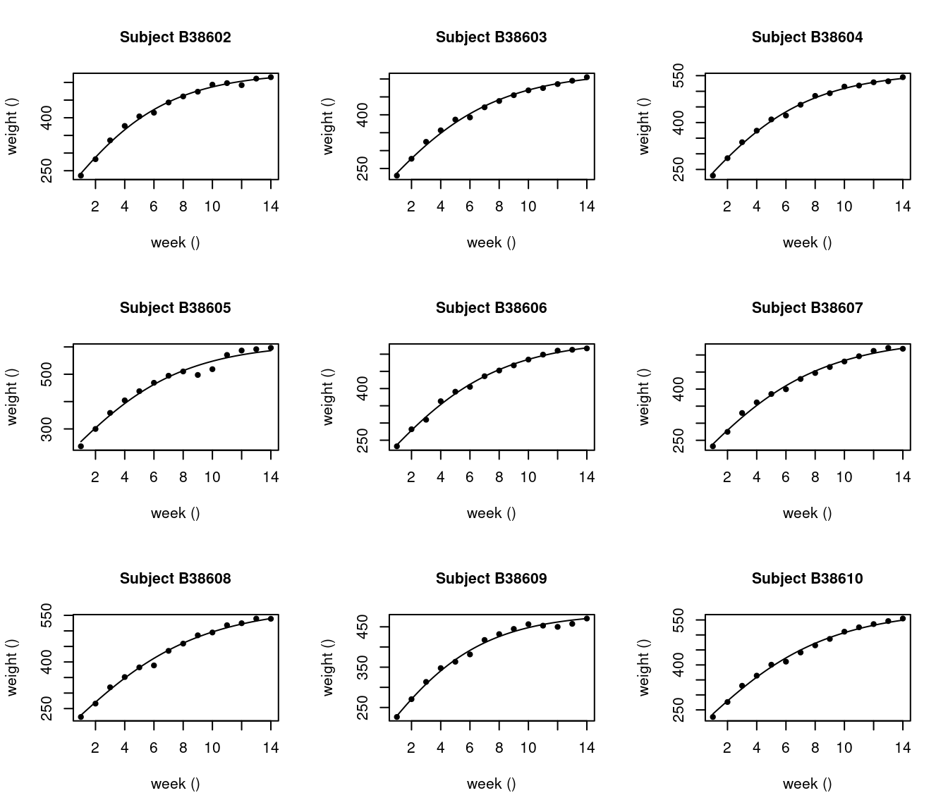
# Diagnostic plot: observations versus population predictions
saemix.plot.obsvspred(NLMM_gompertz_fit)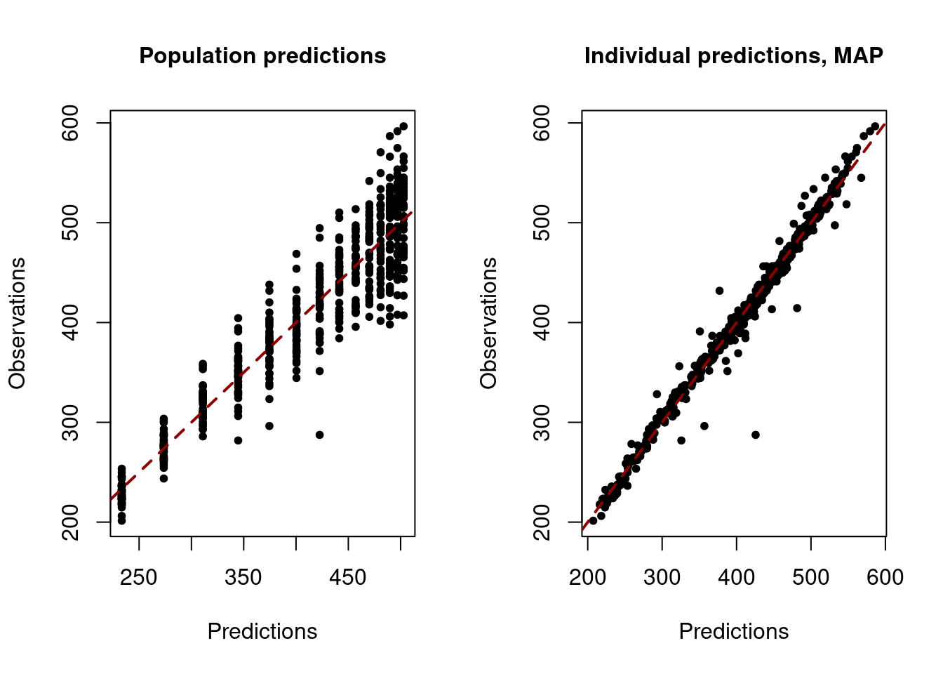
# Scatter plot of residuals
saemix.plot.scatterresiduals(NLMM_gompertz_fit, level=1)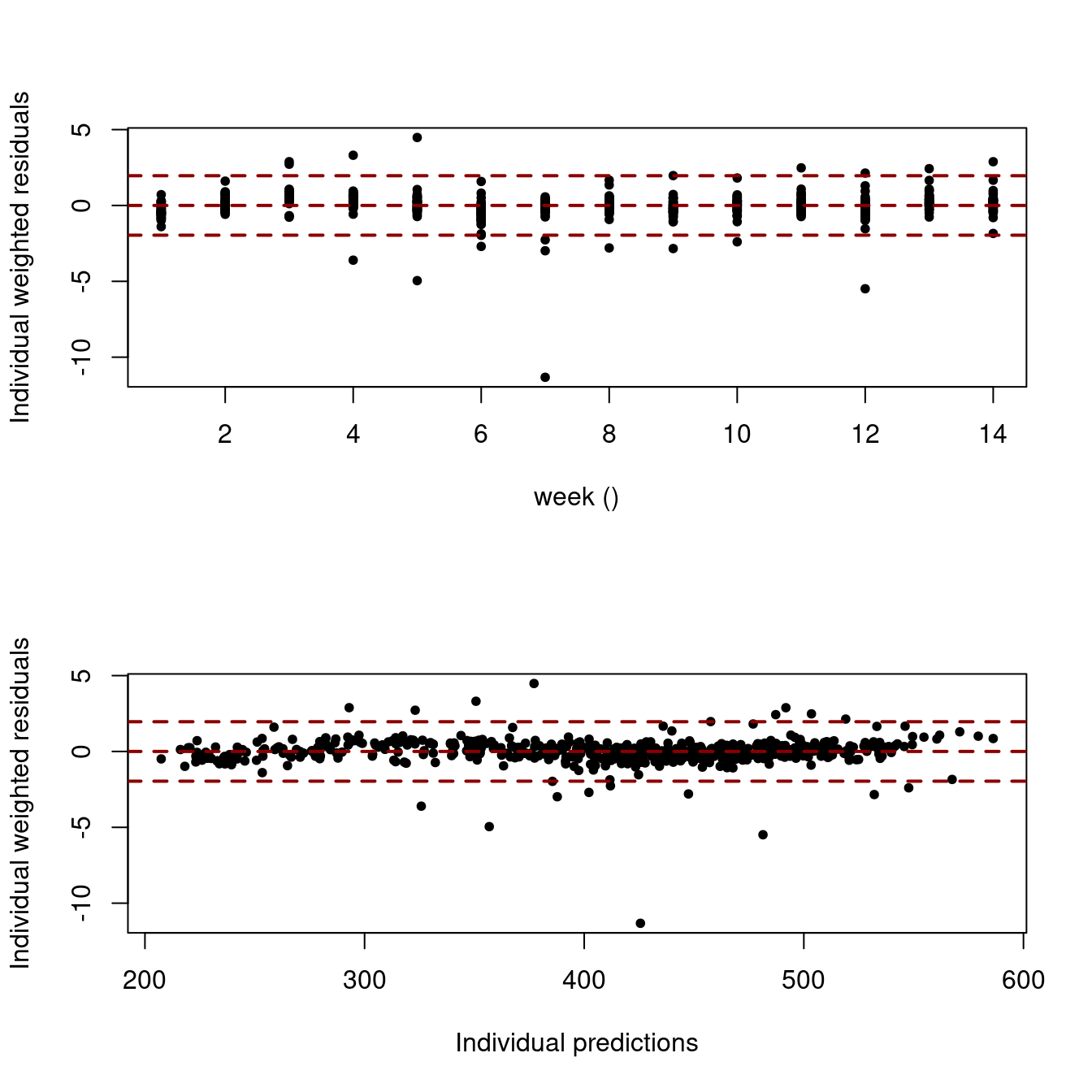
3.1.5 Correlation matrix of the estimates
fim <- NLMM_gompertz_fit@results@fim # Fisher information matrix
cov_hat <- solve(fim)                # covariance matrix of the estimates
d <- sqrt(diag(cov_hat))             # s.e. of the estimates
corrplot(cov_hat / (d %*% t(d)), type = 'upper', diag = FALSE)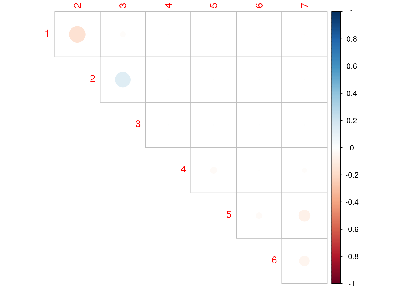
cov_hat / (d %*% t(d)) # correlation matrix of the estimates [,1] [,2] [,3] [,4] [,5] [,6]
[1,] 1.00000000 -0.1521259 -0.01686904 0.0000000000 0.00000000 0.0000000000
[2,] -0.15212594 1.0000000 0.13204038 0.0000000000 0.00000000 0.0000000000
[3,] -0.01686904 0.1320404 1.00000000 0.0000000000 0.00000000 0.0000000000
[4,] 0.00000000 0.0000000 0.00000000 1.0000000000 -0.02345447 -0.0004675813
[5,] 0.00000000 0.0000000 0.00000000 -0.0234544744 1.00000000 -0.0209439728
[6,] 0.00000000 0.0000000 0.00000000 -0.0004675813 -0.02094397 1.0000000000
[7,] 0.00000000 0.0000000 0.00000000 -0.0114581739 -0.07639522 -0.0581498297
[,7]
[1,] 0.00000000
[2,] 0.00000000
[3,] 0.00000000
[4,] -0.01145817
[5,] -0.07639522
[6,] -0.05814983
[7,] 1.000000003.2 Questions
Fit the same model to the same data, assuming different population parameters for the control and GMO groups. Can we conclude that the regime has an effect on the growth of the 11% male rats?
Use an asymptotic regression model f(t) = w_{\infty} + (w_0 -w_{\infty})e^{-k\,t} to test the effect of the regime on the growth of the 11% male rats.
Should we accept the hypothesis that the random effects are uncorrelated?
4 References
Séralini, Gilles-Eric, Dominique Cellier, and Joël Spiroux de Vendomois. 2007. “New Analysis of a Rat Feeding Study with a Genetically Modified Maize Reveals Signs of Hepatorenal Toxicity.” Archives of Environmental Contamination and Toxicology 52 (4): 596–602. https://link.springer.com/article/10.1007/s00244-006-0149-5.