LAVA: Recovering Sums of Sparse and Dense Signals

The lava() and group_lava() estimators in quadrupen

Motivation

Classical sparse estimators such as the Lasso assume that the true coefficient vector \(\theta\) is itself sparse: only a few entries are nonzero. This assumption fails when the signal has a mixed structure — a small number of large, identifiable effects superimposed on a broad background of many small effects. In this case neither the Lasso (too sparse) nor ridge regression (too dense) is well-suited.

The LAVA estimator (Chernozhukov, Hansen & Liao, Annals of Statistics, 2017) explicitly decomposes the coefficient vector as

\[\theta = \beta + \delta,\]

where \(\beta\) is the sparse component (penalized by \(\lambda_1 \|\beta\|_1\)) and \(\delta\) is the dense component (penalized by \(\frac{\lambda_2}{2} \delta^\top S\, \delta\)). The joint criterion is

\[\min_{\theta = \beta + \delta} \frac{1}{2n} \|y - X(\beta + \delta)\|^2 + \lambda_1 \|\beta\|_1 + \frac{\lambda_2}{2}\, \delta^\top S\, \delta,\]

where \(S\) is a positive semidefinite structuring matrix (identity by default). By varying \(\lambda_1\) along a regularization path (with \(\lambda_2\) fixed), quadrupen fits this model via lava() and returns an object of class LavaFit that gives access to both components separately.

Setup

library(quadrupen)
library(ggplot2)

Simulation: a mixed sparse + dense signal

We simulate a linear model where the true signal is the sum of a sparse part \(\beta\) (five isolated large effects) and a dense part \(\delta\) (small Gaussian perturbations on every predictor). Neither component alone characterizes the signal.

set.seed(42)
n <- 100
p <- 50

## Sparse component: 5 large effects, the rest zero
beta  <- numeric(p)
beta[c(5, 15, 25, 35, 45)] <- c(3, -3, 3, -3, 3)

## Dense component: small effects on all predictors
delta <- rnorm(p, mean = 0, sd = 0.2)

## Total signal
theta <- beta + delta

## Predictors with moderate AR(1) correlation
rho   <- 0.5
Sigma <- toeplitz(rho^(0:(p - 1)))
X     <- matrix(rnorm(n * p), n, p) %*% chol(Sigma)
y     <- X %*% theta + rnorm(n, sd = 2)

df_truth <- data.frame(
  index     = rep(1:p, 3),
  value     = c(beta, delta, theta),
  component = factor(
    rep(c("Sparse (β)", "Dense (δ)", "Total (θ = β + δ)"), each = p),
    levels = c("Sparse (β)", "Dense (δ)", "Total (θ = β + δ)")
  )
)

ggplot(df_truth, aes(x = index, y = value, fill = component)) +
  geom_col() +
  facet_wrap(~ component, ncol = 1, scales = "free_y") +
  scale_fill_manual(values = c("#56B4E9", "#E69F00", "#009E73"), guide = "none") +
  labs(x = "Predictor index", y = "Value",
       title = "True signal decomposition") +
  theme_bw()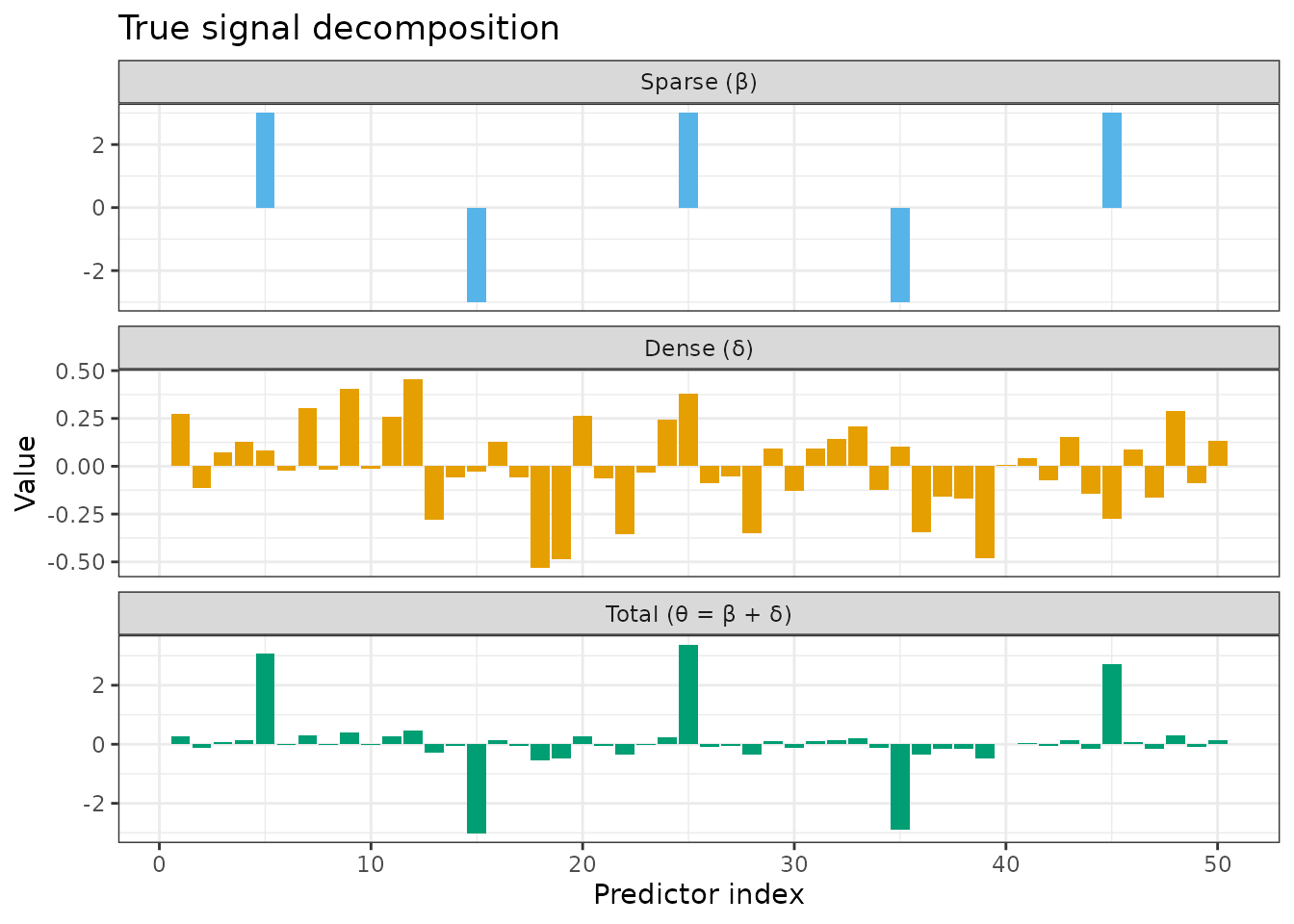

Fitting with lava()

lava() takes the same interface as sparse_lm(). The lambda2 argument controls the ridge-like penalty on the dense component.

fit_lava <- lava(X, y, lambda2 = 1)
fit_lava
#> Linear regression with Lava penalizer.
#> - number of coefficients: 50 + intercept
#> - lambda regularization: 100 points from 16.1 to 0.161
#> - gamma regularization: 1

The returned object is an R6 instance of class LavaFit, inheriting from QuadrupenFit. In addition to all the standard fields and methods ($coefficients, $criteria(), $cross_validate(), etc.), it exposes two component-specific fields:

• $sparse_coef: the sparse part \(\hat\beta\) — a \(p \times |\lambda_1|\) matrix along the path.
• $dense_coef: the dense part \(\hat\delta = \hat\theta - \hat\beta\) — same dimensions.

Regularization paths by component

$plot_path() accepts a component argument ("both", "sparse", "dense") to display each part of the decomposition independently.

fit_lava$plot_path(component = "both",   labels = NULL)
fit_lava$plot_path(component = "sparse", labels = NULL)
fit_lava$plot_path(component = "dense",  labels = NULL)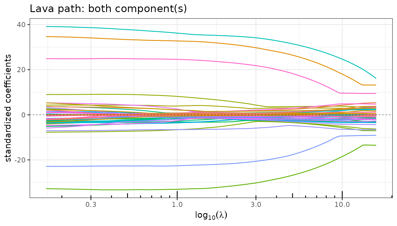

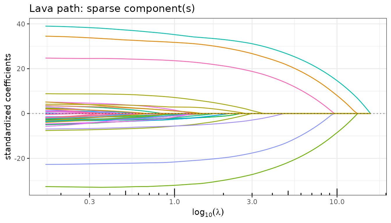
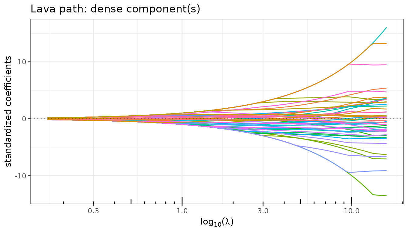
As \(\lambda_1\) increases (right to left on the path):

• The sparse path shows the usual Lasso-like variable selection: large effects enter early and small ones remain zero.
• The dense path is smooth and non-zero everywhere: the ridge penalty ensures that \(\hat\delta\) is distributed across all predictors.
• The total path combines both: it never reaches exactly zero because the dense component picks up residual signal.

Model Selection

Let us plot the information criteria along the path. The BIC and eBIC select a model with a couple of large effects in the sparse part, while AIC selects a more complex model with more non-zero entries in the sparse component. mBIC is more conservative, as expected.

fit_lava$information_criteria$plot(c("AIC", "BIC", "eBIC", "mBIC"))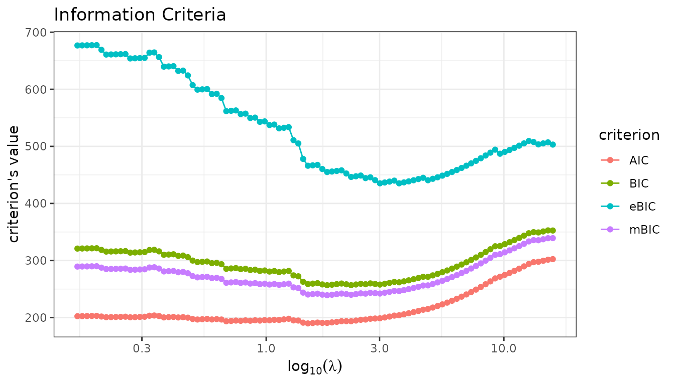

Model extraction and decomposition

$get_model() extracts the total estimated coefficient \(\hat\theta\) at a selected \(\lambda_1\). The corresponding sparse and dense components can be recovered from $sparse_coef and $dense_coef at the same index.

idx <- fit_lava$get_model("BIC", type = "index")

theta_hat <- fit_lava$get_model("BIC")[-1]          # drop intercept
beta_hat  <- as.numeric(fit_lava$sparse_coef[, idx])
delta_hat <- as.numeric(fit_lava$dense_coef[, idx])

cat("Non-zero entries in sparse component (BIC):",
    sum(beta_hat != 0), "\n")
#> Non-zero entries in sparse component (BIC): 12
cat("Non-zero entries in dense component (BIC): ",
    sum(delta_hat != 0), "\n")
#> Non-zero entries in dense component (BIC):  50
cat("Positions with |beta_hat| > 1:",
    which(abs(beta_hat) > 1), "\n")
#> Positions with |beta_hat| > 1: 5 15 25 35 45

The sparse component correctly locates the five large effects — those with |beta_hat| > 1 match the true positions exactly. The dense component is non-zero everywhere, absorbing the background of small signals.

Comparing estimators

We compare LAVA against the Lasso and Elastic-net at their BIC-selected models. In the LAVA panel, bars are split into two layers drawn with geom_col: the total estimate \(\hat\theta = \hat\beta + \hat\delta\) is drawn first (pink, dense component), and the sparse component \(\hat\beta\) is overlaid on top (green). The remaining pink portion at the tips of active bars represents the dense contribution \(\hat\delta\); the small pink bars at inactive positions are the dense signal alone.

fit_lasso <- lasso(X, y)
fit_enet  <- elastic_net(X, y, lambda2 = 1)

get_coef <- function(fit) {
  b <- fit$get_model("BIC")
  if ("Intercept" %in% names(b)) b <- b[-1]
  as.numeric(b)
}

method_levels <- c("True signal", "Lasso (BIC)", "Elastic-net (BIC)", "LAVA (BIC)")

## Non-LAVA panels: one bar per predictor
df_base <- rbind(
  data.frame(method = "True signal",       index = 1:p,
             value = theta,                fill_grp = "True signal"),
  data.frame(method = "Lasso (BIC)",       index = 1:p,
             value = get_coef(fit_lasso),  fill_grp = "Lasso"),
  data.frame(method = "Elastic-net (BIC)", index = 1:p,
             value = get_coef(fit_enet),   fill_grp = "Elastic-net")
)
df_base$method <- factor(df_base$method, levels = method_levels)

## LAVA panel: dense total drawn first, sparse component overlaid on top
df_lava_dense <- data.frame(
  method   = factor("LAVA (BIC)", levels = method_levels),
  index    = 1:p,
  value    = as.numeric(theta_hat),
  fill_grp = "LAVA dense (δ̂)"
)
df_lava_sparse <- data.frame(
  method   = factor("LAVA (BIC)", levels = method_levels),
  index    = 1:p,
  value    = beta_hat,
  fill_grp = "LAVA sparse (β̂)"
)

fill_palette <- c(
  "True signal"       = "grey20",
  "Lasso"             = "#56B4E9",
  "Elastic-net"       = "#E69F00",
  "LAVA dense (δ̂)"   = "#CC79A7",
  "LAVA sparse (β̂)"  = "#009E73"
)

ggplot(mapping = aes(x = index, y = value, fill = fill_grp)) +
  geom_col(data = df_base) +
  geom_col(data = df_lava_dense) +
  geom_col(data = df_lava_sparse) +
  facet_wrap(~ method, ncol = 2) +
  scale_fill_manual(
    values = fill_palette,
    breaks = c("LAVA sparse (β̂)", "LAVA dense (δ̂)"),
    name   = "LAVA decomposition"
  ) +
  labs(x = "Predictor index", y = "Estimated coefficient",
       title = "Coefficient recovery: Lasso vs. Elastic-net vs. LAVA") +
  theme_bw() +
  theme(legend.position = "bottom")
#> Warning in min(x): no non-missing arguments to min; returning Inf
#> Warning in max(x): no non-missing arguments to max; returning -Inf
#> Warning in min(x): no non-missing arguments to min; returning Inf
#> Warning in max(x): no non-missing arguments to max; returning -Inf
#> Warning in min(x): no non-missing arguments to min; returning Inf
#> Warning in max(x): no non-missing arguments to max; returning -Inf
#> Warning in min(x): no non-missing arguments to min; returning Inf
#> Warning in max(x): no non-missing arguments to max; returning -Inf
#> Warning in min(x): no non-missing arguments to min; returning Inf
#> Warning in max(x): no non-missing arguments to max; returning -Inf
#> Warning in min(x): no non-missing arguments to min; returning Inf
#> Warning in max(x): no non-missing arguments to max; returning -Inf
#> Warning in min(x): no non-missing arguments to min; returning Inf
#> Warning in max(x): no non-missing arguments to max; returning -Inf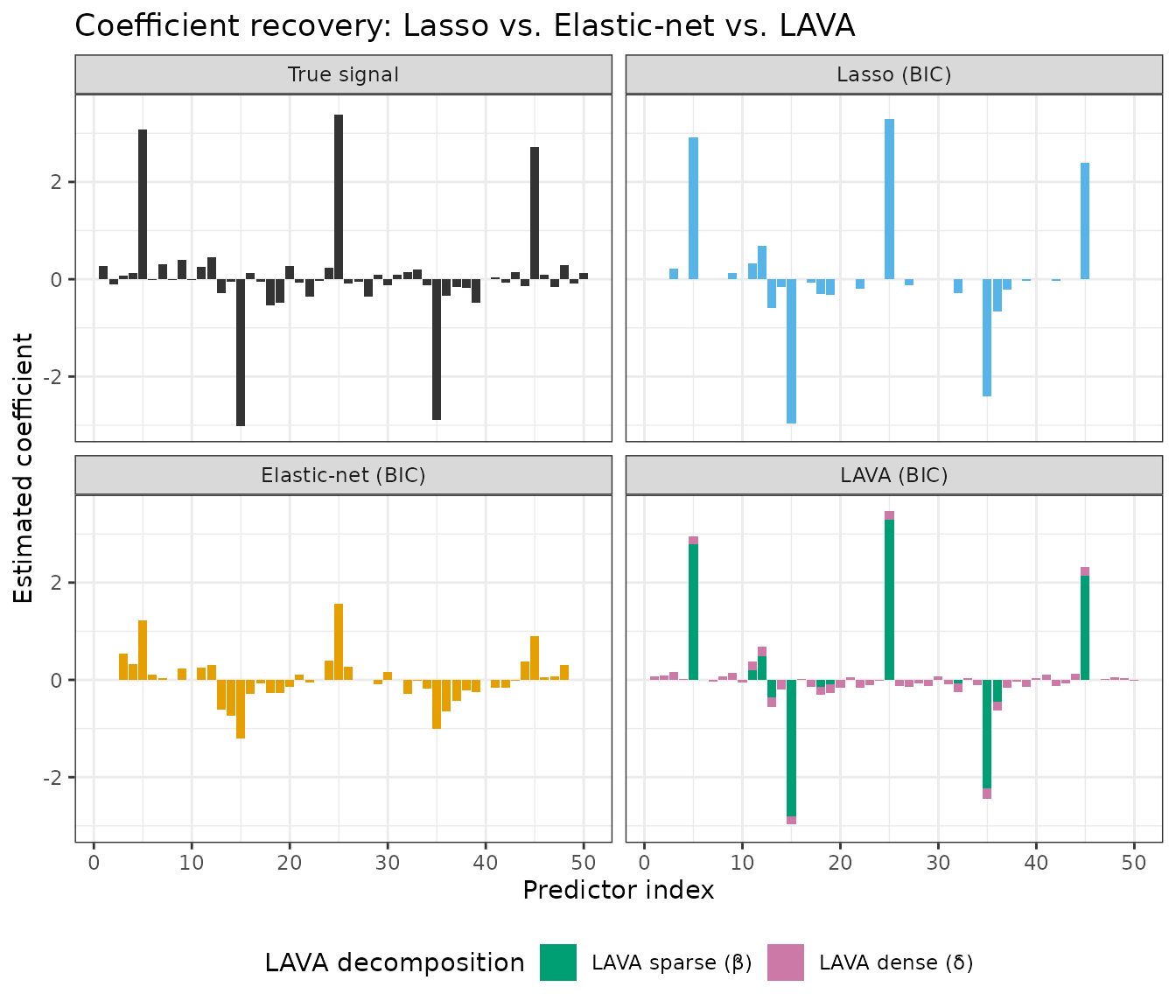

• The Lasso selects a handful of predictors but cannot represent the dense background.
• The Elastic-net spreads a small weight across more predictors, but conflates the two structural components.
• LAVA explicitly decomposes the signal: the green bars identify the large sparse effects precisely; the pink portions (small rims at active positions, full bars at inactive positions) capture the diffuse dense background.

Cross-validation

$cross_validate() works identically to the other QuadrupenFit subclasses.

set.seed(42)
fit_lava$cross_validate(K = 10, verbose = FALSE)
fit_lava$plot(type = "crossval")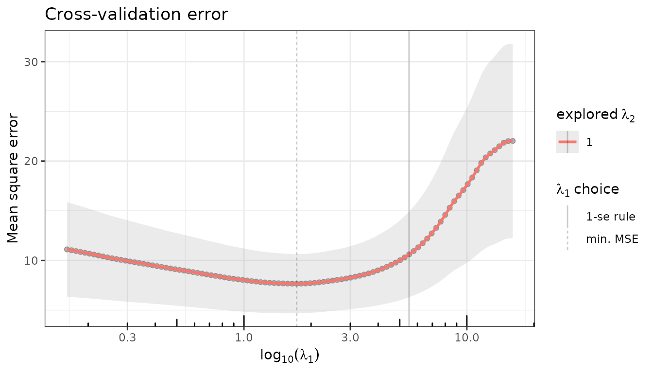

set.seed(42)
fit_lasso$cross_validate(K = 10, verbose = FALSE)
fit_enet$cross_validate(K = 10, verbose = FALSE)

idx_cv   <- fit_lava$get_model("CV_min", type = "index")
beta_cv  <- as.numeric(fit_lava$sparse_coef[, idx_cv])
cat("Non-zero entries in sparse component (CV_min):",
    sum(beta_cv != 0), "\n")
#> Non-zero entries in sparse component (CV_min): 13
cat("Positions with |beta_cv| > 1:",
    which(abs(beta_cv) > 1), "\n")
#> Positions with |beta_cv| > 1: 5 15 25 35 45

---

Group LAVA: group-sparse + dense decomposition

group_lava() extends LAVA by replacing the element-wise \(\ell_1\) penalty on \(\beta\) with a group-wise mixed norm \(\Omega_g(\beta)\):

\[\min_{\theta = \beta + \delta} \frac{1}{2n} \|y - X(\beta + \delta)\|^2 + \lambda_1\, \Omega_g(\beta) + \frac{\lambda_2}{2}\, \delta^\top S\, \delta.\]

This is appropriate when the sparse component has group structure: entire groups of predictors are either active or silent. The type argument selects the group norm (\(\ell_1/\ell_2\) by default, or \(\ell_1/\ell_\infty\)).

Simulation with a group-sparse signal

## 5 groups of 10 predictors; groups 2 and 4 are active in the sparse part
group  <- rep(1:5, each = 10)
beta_g <- rep(c(0, 2, 0, -2, 0), each = 10)
delta_g <- rnorm(p, mean = 0, sd = 0.2)
theta_g <- beta_g + delta_g

y2 <- X %*% theta_g + rnorm(n, sd = 2)

group_names <- paste0("grp", 1:5)
var_labels  <- group_names[group]

Fitting

fit_gl <- group_lava(X, y2, group = group, lambda2 = 1)
fit_gl
#> Linear regression with group Lava l1/l2 penalizer.
#> - number of coefficients: 50 + intercept
#> - lambda regularization: 100 points from 14.9 to 0.149
#> - gamma regularization: 1

Paths of the sparse and dense components

fit_gl$plot_path(component = "sparse", labels = var_labels)
fit_gl$plot_path(component = "dense",  labels = var_labels)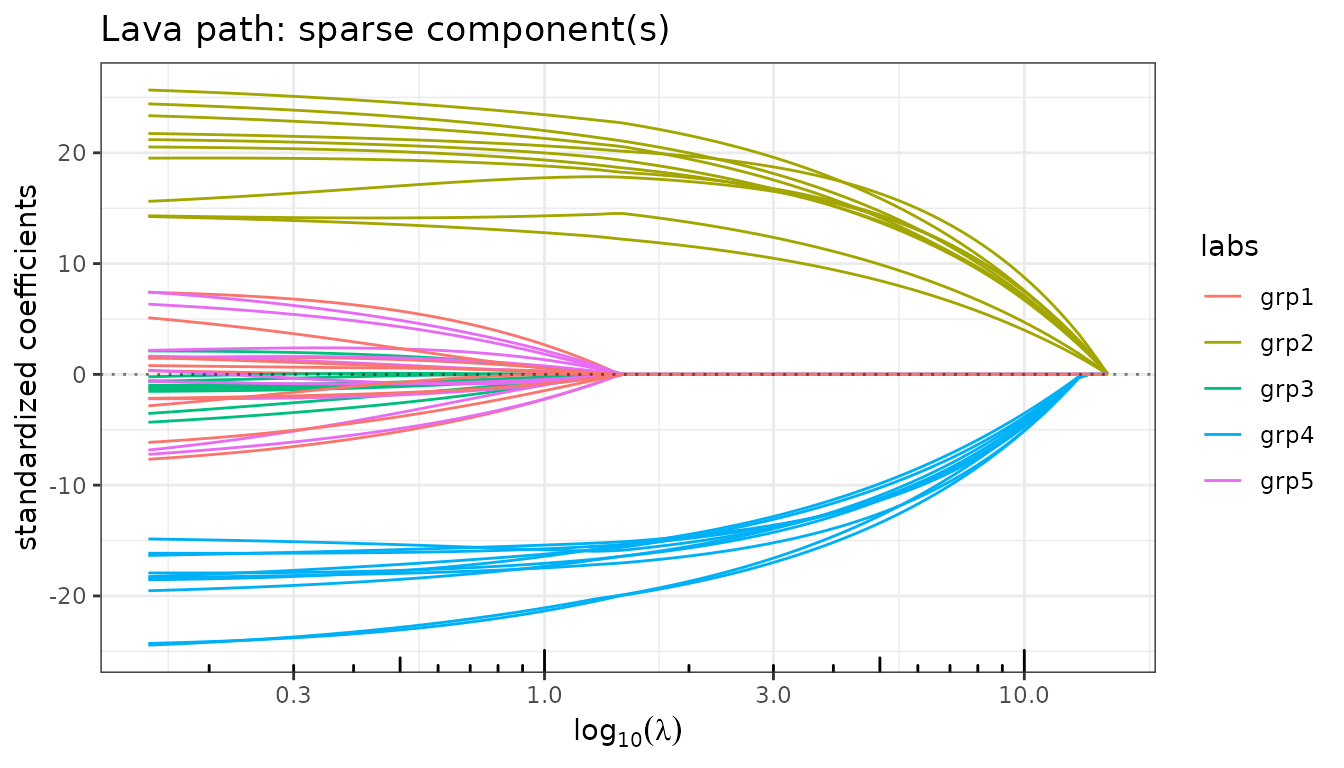

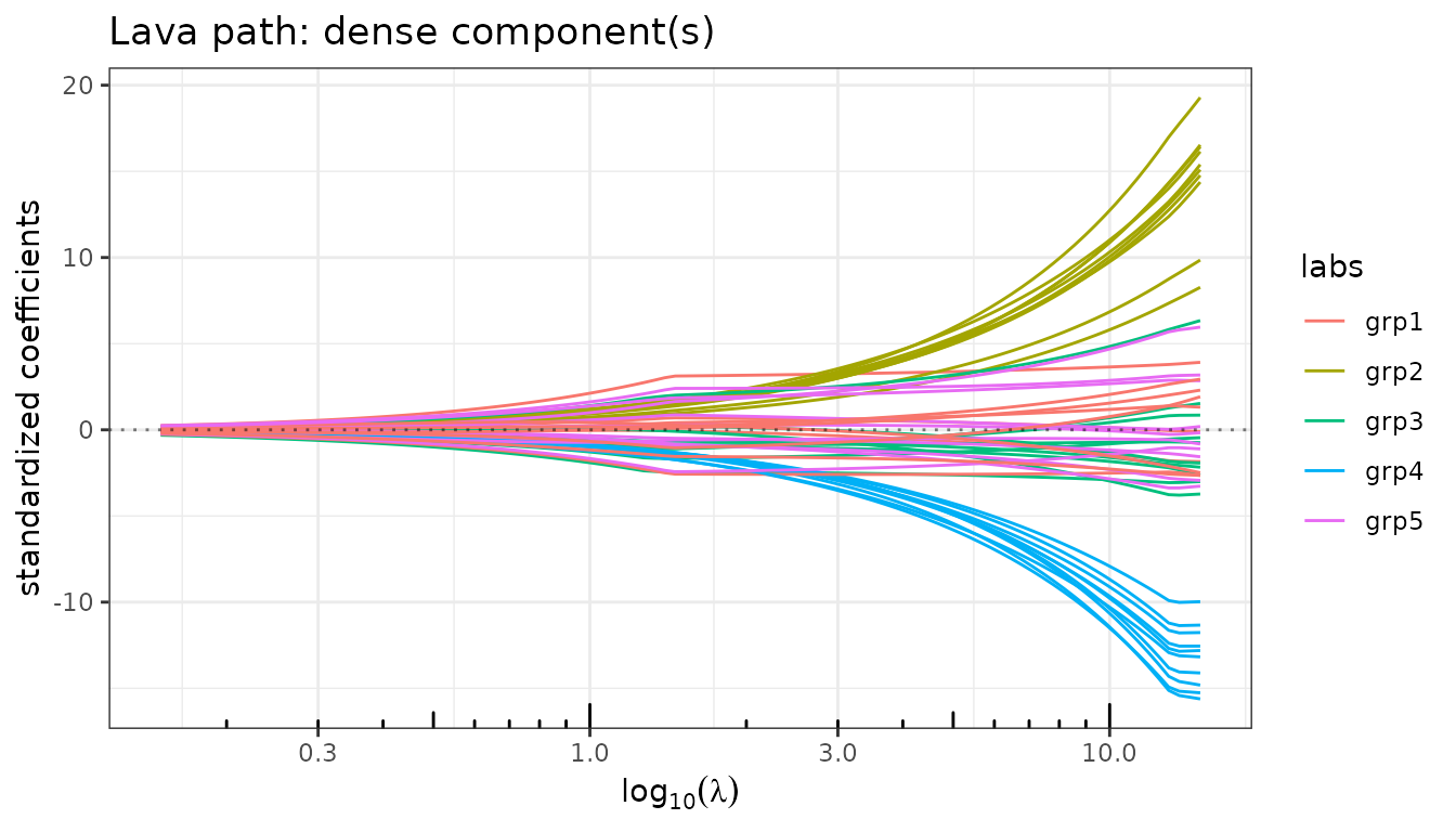
The sparse path shows entire groups entering the model simultaneously (Group Lasso behaviour), while the dense path remains diffuse and non-zero everywhere.

Model selection

For group selection problems, eBIC (which carries a stronger penalty of \(\log(n) + 2\log(p)\)) is generally more conservative than BIC and better adapted to identifying which groups are truly active.

Group identification

idx_ebic   <- fit_gl$get_model("eBIC", type = "index")
beta_g_hat <- as.numeric(fit_gl$sparse_coef[, idx_ebic])

active_groups <- unique(group[beta_g_hat != 0])
cat("Active groups in sparse component (eBIC):", group_names[active_groups], "\n")
#> Active groups in sparse component (eBIC): grp2 grp4

---

Reference

Chernozhukov, V., Hansen, C., & Liao, Y. (2017). A lava attack on the recovery of sums of dense and sparse signals. The Annals of Statistics, 45(1), 39–76. https://doi.org/10.1214/16-AOS1434