Adjust a lava regularized linear model, that is a lava transformation of the data followed by a (possibly weighted) \(\ell_1\)-norm. The solution path is computed at a grid of values for the \(\ell_1\)-penalty. See details for the criterion optimized.
Usage
lava(
  x,
  y,
  lambda1 = NULL,
  lambda2 = 1,
  weights = rep(1, nrow(x)),
  penscale = rep(1, ncol(x)),
  struct = Matrix::Diagonal(ncol(x), 1),
  intercept = TRUE,
  normalize = TRUE,
  refit = FALSE,
  nlambda1 = ifelse(is.null(lambda1), 100, length(lambda1)),
  minratio = 0.01,
  maxfeat = min(nrow(x), ncol(x)),
  beta0 = numeric(ncol(x)),
  control = list()
)
Arguments
- x
matrix of features, possibly sparsely encoded (experimental). Do NOT include intercept. When normalized is
TRUE, coefficients will then be rescaled to the original scale.- y
response vector.
- lambda1
sequence of decreasing \(\ell_1\)-penalty levels. If
NULL(the default), a vector is generated withnlambda1entries, starting from a guessed levellambda1.maxwhere only the intercept is included, then shrunken tominratio*lambda1.max.- lambda2
real scalar; tunes the \(\ell_2\) penalty in the Elastic-net. Default is 0.01. Set to 0 to recover the Lasso.
- weights
vector with real positive values that weight the observations (like in weighted least square). Default sets all weights to 1.
- penscale
vector with real positive values that weight the penalty of each feature. Default sets all weights to 1.
- struct
matrix structuring the coefficients, possibly sparsely encoded. Must be at least positive semidefinite (this is checked internally). If
NULL(the default), the identity matrix is used. See details below.- intercept
logical; indicates if an intercept should be included in the model. Default is
TRUE.- normalize
logical; indicates if variables should be normalized to have unit L2 norm before fitting. Default is
TRUE.- refit
logical: indicates if the non null coefficients should be refit to avoid excessive bias. Default is FALSE. Can be changed later (both raw and refit coefficients are stored).
- nlambda1
integer that indicates the number of values to put in the
lambda1vector. Ignored iflambda1is provided.- minratio
minimal value of \(\ell_1\)-part of the penalty that will be tried, as a fraction of the maximal
lambda1value. A too small value might lead to instability at the end of the solution path corresponding to smalllambda1combined with \(\lambda_2=0\). The default value tries to avoid this, adapting to the '\(n<p\)' context. Ignored iflambda1is provided.- maxfeat
integer; limits the number of features ever to enter the model; i.e., non-zero coefficients for the Elastic-net: the algorithm stops if this number is exceeded and
lambda1is cut at the corresponding level. Default ismin(nrow(x),ncol(x))for smalllambda2(<0.01) andmin(4*nrow(x),ncol(x))otherwise. Use with care, as it considerably changes the computation time.- beta0
a starting point for the vector of parameter. By default, will initialized zero. May save time in some situation.
- control
list of argument controlling low level options of the algorithm –use with care and at your own risk– :
verbose: integer; activate verbose mode –this one is not too risky!– set to0for no output;1for warnings only, and2for tracing the whole progression. Default is1. Automatically set to0when the method is embedded within cross-validation or stability selection.timer: logical; use to record the timing of the algorithm. Default isFALSE.maxiterthe maximal number of iteration used in the active set algorithm to solve the problem for a given value of lambda1 . Default is 50.methoda string for the underlying solver used. Either"quadra","fista"or"pgd". Default is"quadra".factmatBoolean indicating if matrix factorization should be used to solve the sub-system. IfTRUE(the default), a Cholesky decomposition is maintained along the path. IfFALSE, the sub-system are solved with a conjugate gradient algorithm.thresholda threshold for convergence. The algorithm stops when the optimality conditions are fulfill up to this threshold. Default is1e-6.monitorindicates if a monitoring of the convergence should be recorded, by computing a lower bound between the current solution and the optimum: when'0'(the default), no monitoring is provided; when'1', the bound derived in Grandvalet et al. is computed; when'>1', the Fenchel duality gap is computed along the algorithm.
Value
an object with class QuadrupenFit.
an object with class LavaFit, inheriting from QuadrupenFit.
Details
The optimized criterion is the following: βhatλ1 = argminθ = β+δ 1/2n RSS(β + δ) + λ1 | β |1 + λ/2 2 δT S δ, .
References
Chernozhukov, Victor, Christian Hansen, and Yuan Liao. "A lava attack on the recovery of sums of dense and sparse signals." The Annals of Statistics (2017): 39-76. doi:10.1214/16-AOS1434
Examples
## Simulating multivariate Gaussian with blockwise correlation
## and piecewise constant vector of parameters
beta <- rep(c(0,1,0,-1,0), c(25,10,25,10,25))
delta <- runif(sum(c(25,10,25,10,25)),-.1,.1)
cor <- 0.75
Soo <- toeplitz(cor^(0:(25-1))) ## Toeplitz correlation for irrelevant variables
Sww <- matrix(cor,10,10) ## bloc correlation between active variables
Sigma <- Matrix::bdiag(Soo,Sww,Soo,Sww,Soo)
diag(Sigma) <- 1
n <- 50
x <- as.matrix(matrix(rnorm(95*n),n,95) %*% chol(Sigma))
y <- 10 + x %*% beta + rnorm(n,0,10)
labels <- rep("irrelevant", length(beta))
labels[beta != 0] <- "relevant"
## The solution path of the LAVA
out <- lava(x,y)
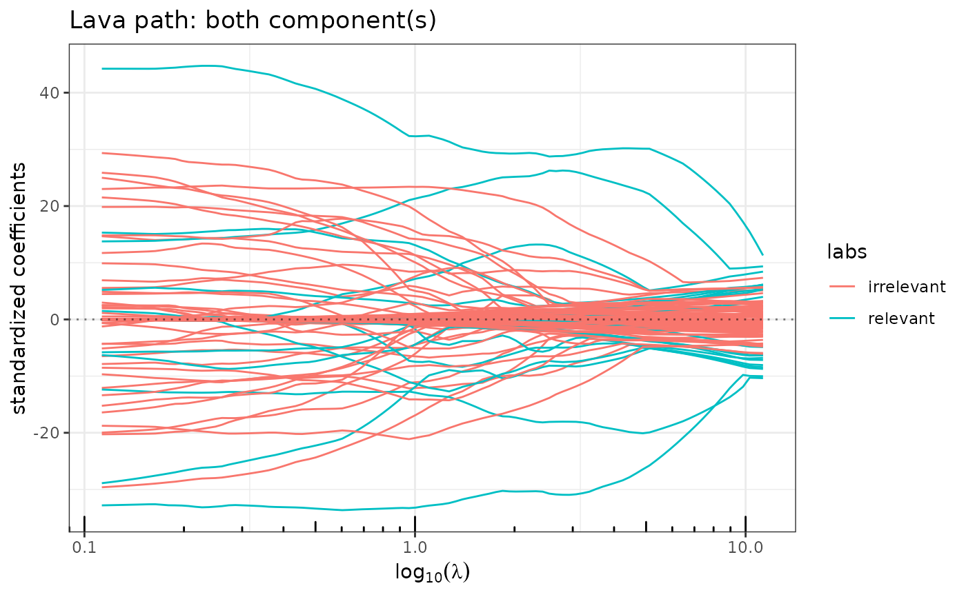
out$plot_path(component = "sparse", labels=labels)
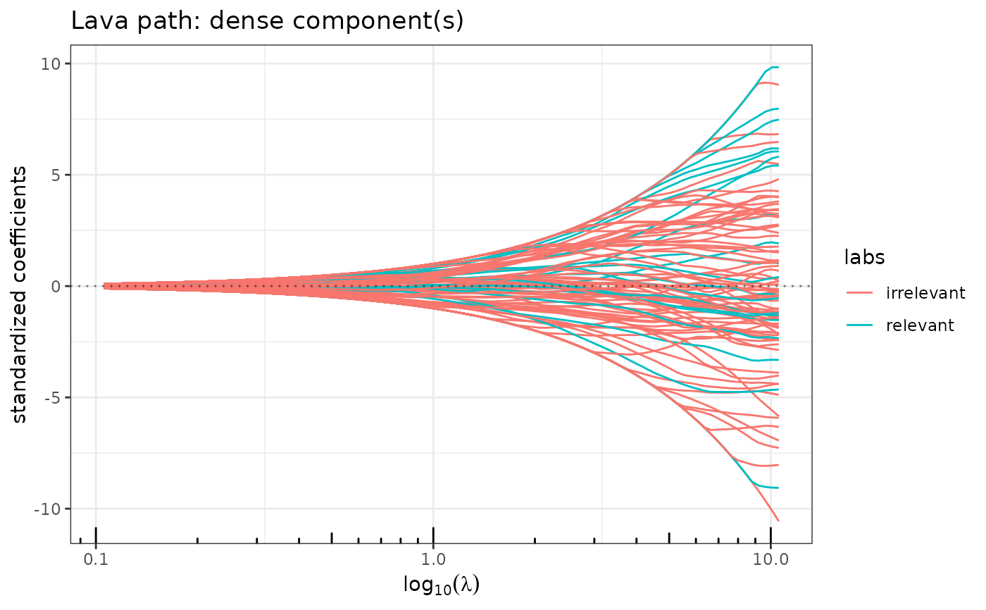
 out$plot_path(component = "dense", labels=labels)