Sparse Linear Regression with Quadrupen

Setup

library(quadrupen)
#> 'quadrupen' package version 1.0-0
data("Birthwt", package = "grpreg")
y <- Birthwt$bwt[-130] ## outlier
X <- Birthwt$X[-130, ]

The Birthwt dataset contains birth weight data with 189 observations and 16 predictors. We use it throughout this vignette to illustrate sparse linear regression.

Fitting sparse linear models

The main entry point is sparse_lm(), which fits a regularization path for several sparse penalties: "l1" (Lasso/Elastic-net), "mcp" (Minimax Concave Penalty) and "scad" (Smoothly Clipped Absolute Deviation). Convenience wrappers lasso(), mcp(), scad() and elastic_net() are also available.

Lasso

fit_lasso <- lasso(X, y, minratio = 1e-2)
fit_lasso
#> Linear regression with L1  penalizer.
#> - number of coefficients: 16 + intercept
#> - lambda regularization: 100 points from 2.78 to 0.0278
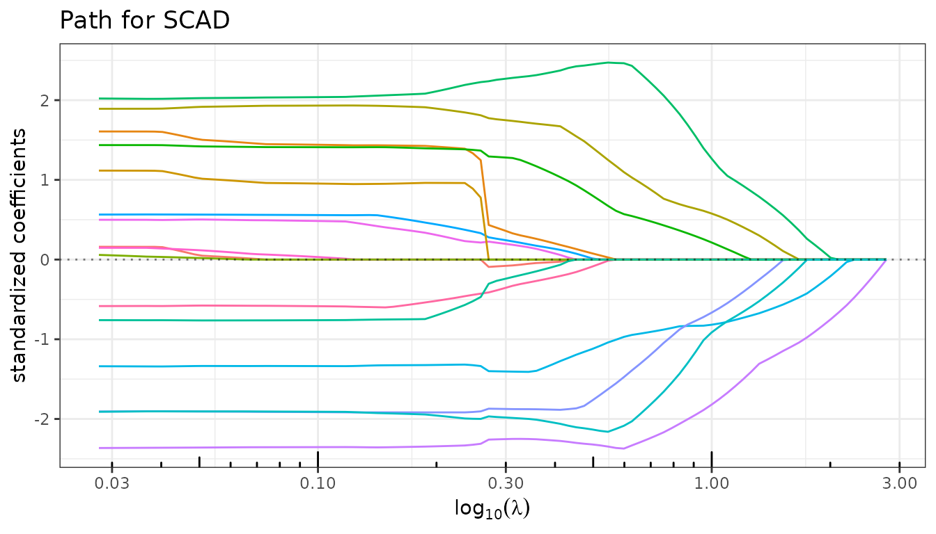
#> - gamma regularization: 0

SCAD

SCAD is a non-convex penalty that matches the Lasso near the origin and tapers to a constant for large coefficients, thereby eliminating shrinkage bias for strong signals. The shape parameter eta must be greater than 2.

fit_scad <- scad(X, y, eta = 4, minratio = 1e-2)
fit_scad
#> Linear regression with SCAD  penalizer.
#> - number of coefficients: 16 + intercept
#> - lambda regularization: 100 points from 2.78 to 0.0278
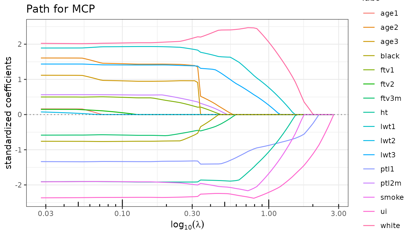
#> - gamma regularization: 0

MCP

MCP applies a linearly diminishing marginal penalty that vanishes once a coefficient exceeds eta × lambda1, yielding near-unbiased estimates for large signals. The shape parameter eta must be greater than 1.

fit_mcp <- mcp(X, y, eta = 3, minratio = 1e-2)
fit_mcp
#> Linear regression with MCP  penalizer.
#> - number of coefficients: 16 + intercept
#> - lambda regularization: 100 points from 2.78 to 0.0278
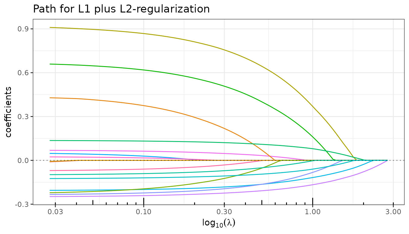
#> - gamma regularization: 0

Elastic-Net

The Elastic-net combines an $\ell_1$ and an $\ell_2$ penalty, trading off sparsity against grouping of correlated predictors. The lambda2 argument controls the ridge component.

fit_enet <- elastic_net(X, y, lambda2 = 1, minratio = 1e-2)
fit_enet
#> Linear regression with L1 plus L2-regularization penalizer.
#> - number of coefficients: 16 + intercept
#> - lambda regularization: 100 points from 2.78 to 0.0278
#> - gamma regularization: 1

Fit objects

All objects returned by sparse_lm() and its wrappers are R6 instances of the class SparseFit, inheriting from QuadrupenFit. These objects (see [QuadrupenFit]) store all data related to the fit, accessible directly via named fields (e.g., fit_lasso$coefficients, fit_lasso$deviance, fit_lasso$degrees_freedom; see str(fit_lasso) and the documentation).

They also provide methods for visualizing and analyzing the fit, and for pursuing complementary analyses such as model selection, cross-validation, and stability selection. For users unfamiliar with R6 classes, S3 methods are exported for the most common operations (e.g., plot(fit_lasso) is equivalent to fit_lasso$plot()), but the R6 methods expose more options.

Regularization paths

$plot_path() (or plot(fit, type = "path")) displays how coefficients evolve along the penalty path.

fit_lasso$plot_path(xvar="fraction", log_scale = FALSE)
fit_mcp$plot_path(labels = colnames(X))
fit_scad$plot_path()
fit_enet$plot_path(standardize=FALSE)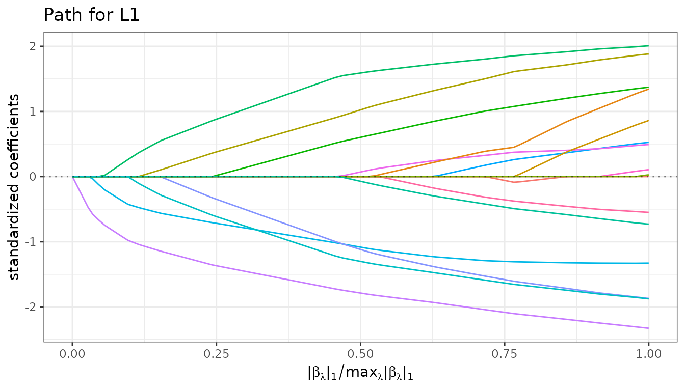

Information criteria

$criteria() computes AIC, BIC, mBIC, eBIC and GCV from the estimated degrees of freedom, storing the result as an [InformationCriteria] R6 object in the field $information_criteria of the current fit. This method is called automatically during fitting (sparse_lm() or any wrapper) at no additional computational cost, so users rarely need to invoke it manually — the main exception being when a custom penalty term is desired.

fit_lasso$criteria()

fit_lasso$plot(type = "criteria")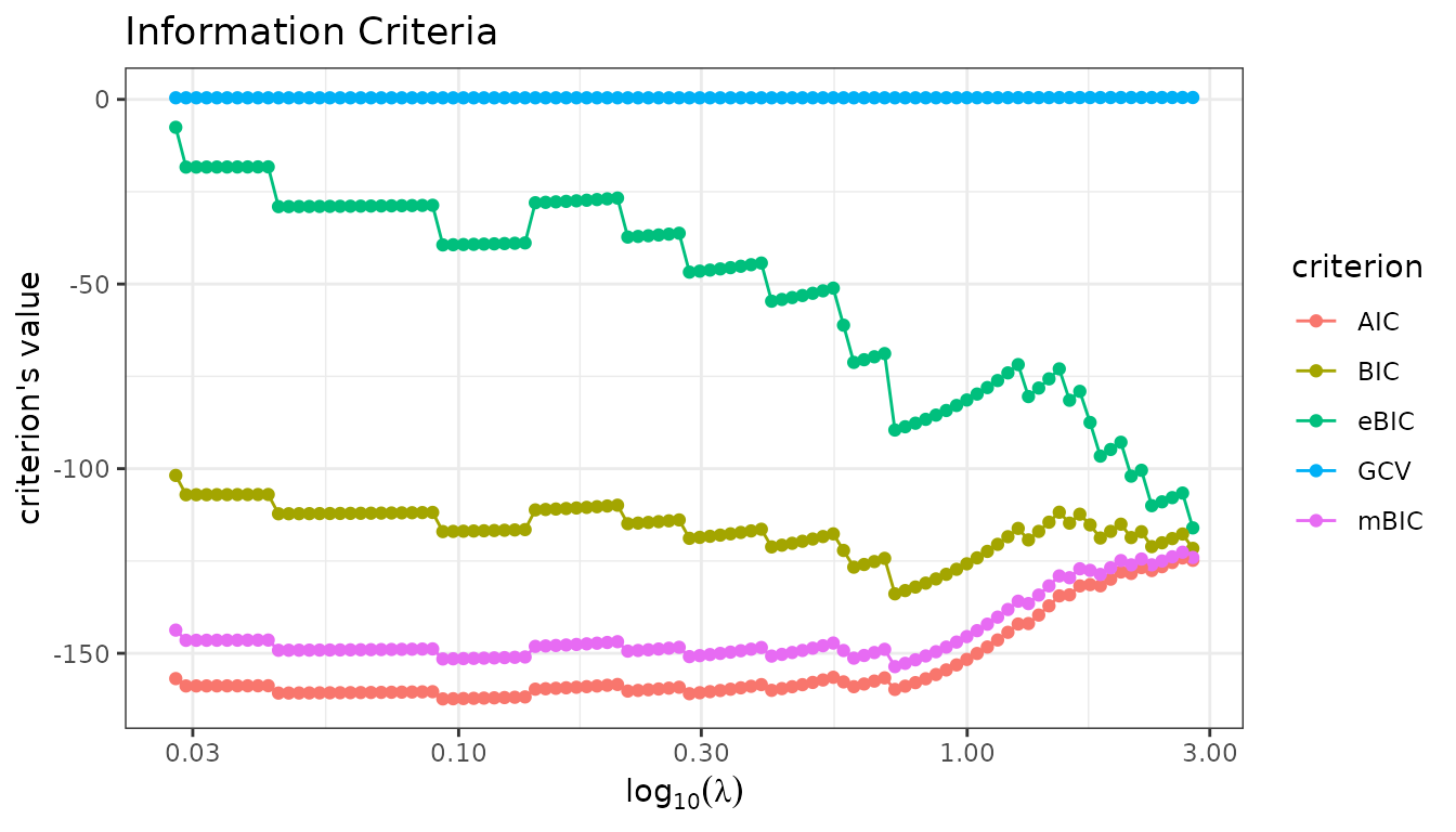

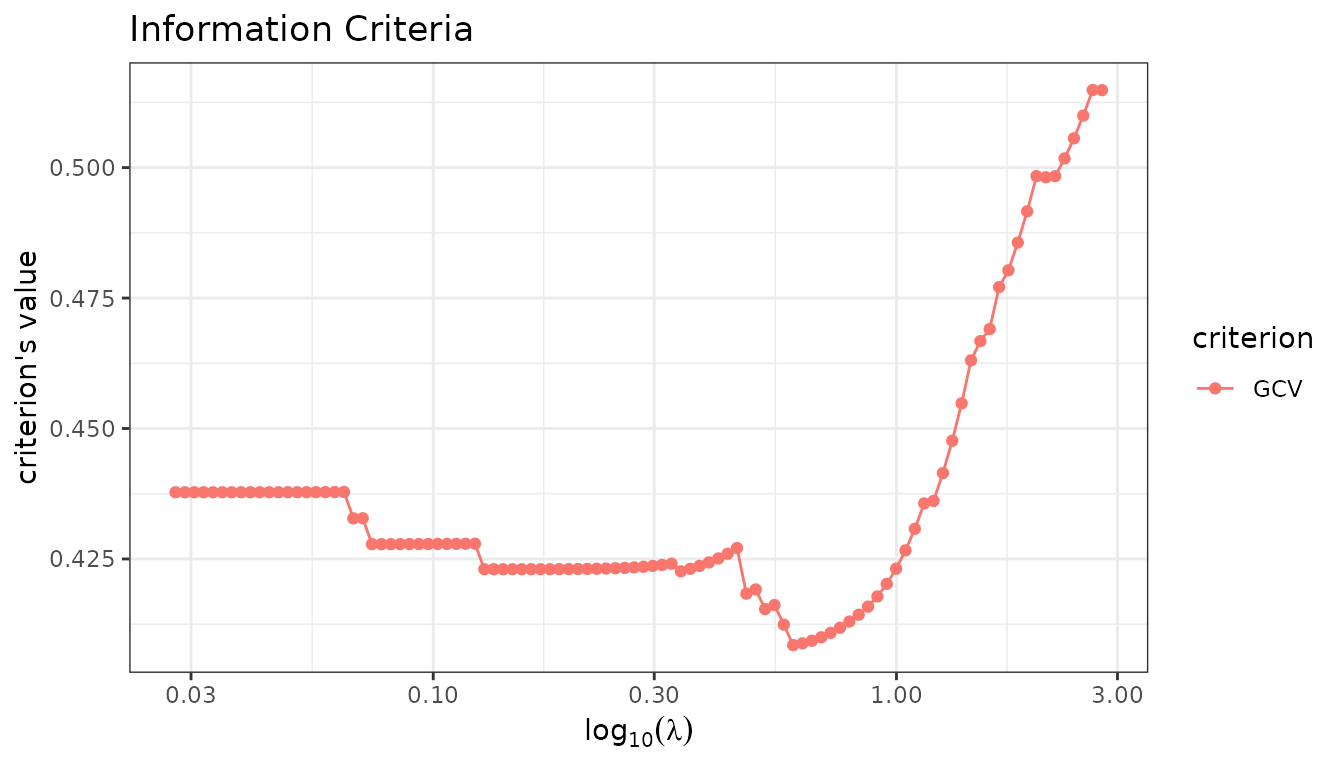
For greater flexibility, use the plot method of the InformationCriteria object directly to select which criteria to display:

fit_lasso$information_criteria$plot(c("AIC", "BIC", "mBIC"))
fit_mcp$information_criteria$plot("GCV")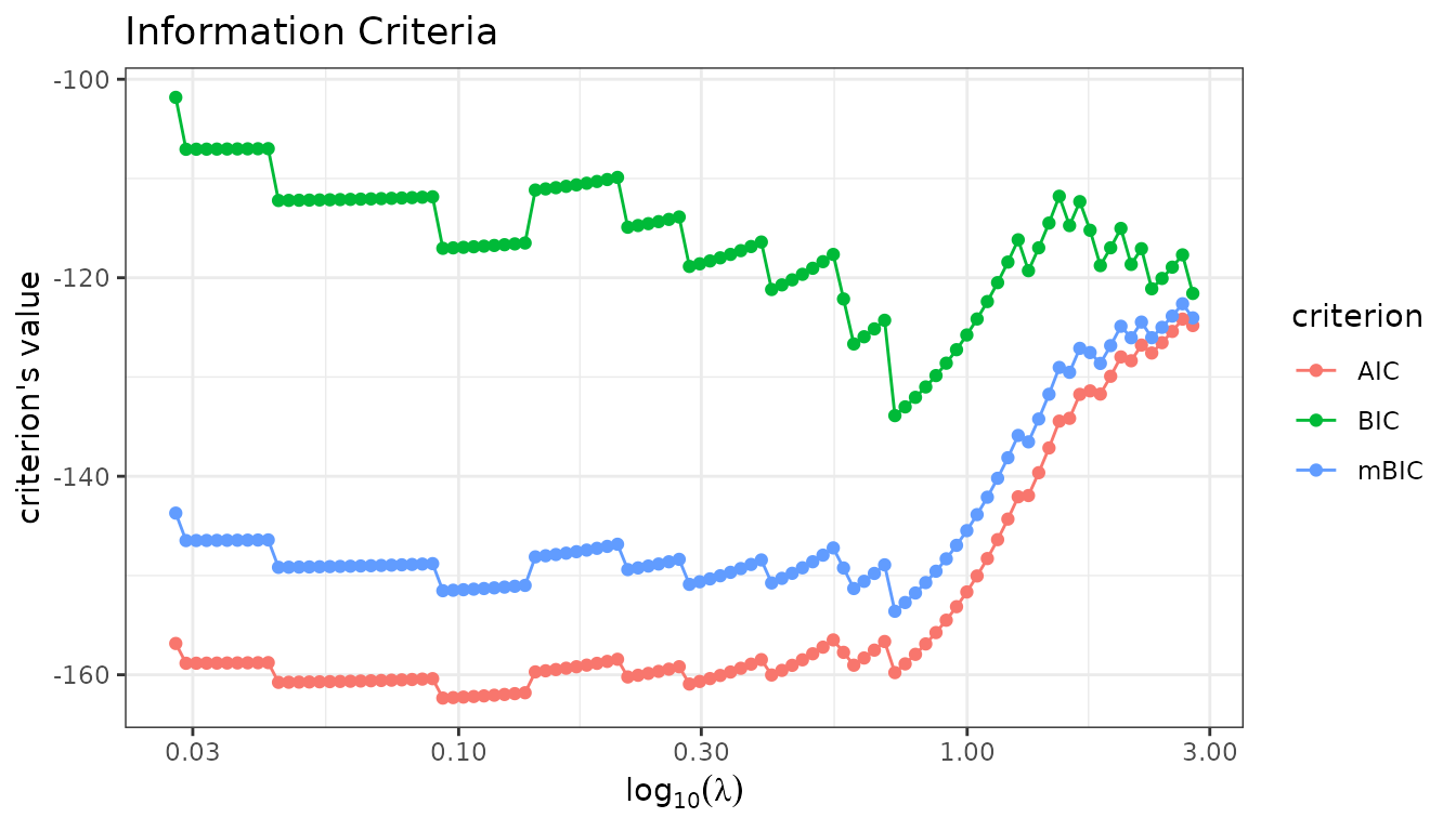

Model extraction

$get_model() extracts the coefficient vector selected by a given criterion.

coef_lasso_bic <- fit_lasso$get_model("BIC")
coef_mcp_bic   <- fit_mcp$get_model("BIC")

cat("Non-zero Lasso coefficients (BIC):\n")
#> Non-zero Lasso coefficients (BIC):
print(coef_lasso_bic[coef_lasso_bic != 0])
#>  Intercept       lwt1       lwt3      white      smoke       ptl1         ht 
#>  2.9931326  0.9025747  0.5131904  0.2216380 -0.1817029 -0.2217365 -0.2969746 
#>         ui 
#> -0.3530479

cat("\nNon-zero MCP coefficients (BIC):\n")
#> 
#> Non-zero MCP coefficients (BIC):
print(coef_mcp_bic[coef_mcp_bic != 0])
#>  Intercept       lwt1       lwt3      white      smoke       ptl1         ht 
#>  3.0186084  1.5356100  0.8812085  0.3530156 -0.3138259 -0.2674971 -0.5596069 
#>         ui 
#> -0.4685982

An existing lambda value can also be passed directly:

lambda_lasso <- fit_lasso$major_tuning
coef_lasso_lambda <- fit_lasso$get_model(lambda_lasso[18])

cat("Non-zero Lasso coefficients for lambda = ", round(lambda_lasso[18], 2), "\n")
#> Non-zero Lasso coefficients for lambda =  1.26
print(coef_lasso_lambda[coef_lasso_lambda != 0])
#>     Intercept          lwt1          lwt3         white         smoke 
#>  2.9725364689  0.3611176526  0.0005800756  0.1252915157 -0.0885736060 
#>          ptl1            ht            ui 
#> -0.1545302819 -0.0972542515 -0.2777916481

Cross-validation

$cross_validate() performs K-fold cross-validation over the penalty grid, storing the result as a [CrossValidation] R6 object in the field $cross_validation of the current fit.

set.seed(42)
fit_lasso$cross_validate(K = 10, verbose = FALSE)
fit_mcp$cross_validate(K = 10, verbose = FALSE)

fit_lasso$plot(type = "crossval")
fit_mcp$plot(type = "crossval")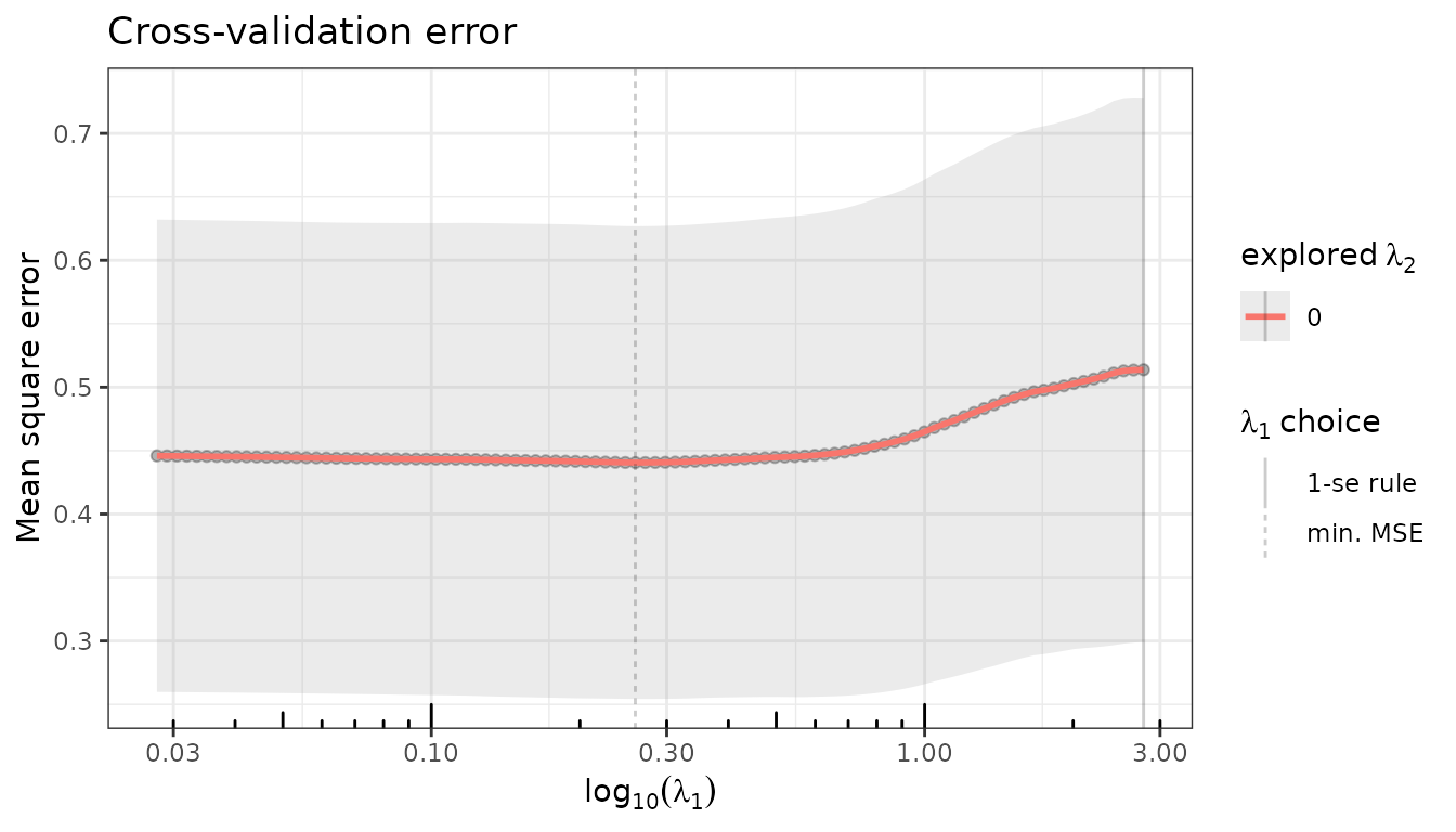

Model selection using the CV-minimizing penalty:

coef_lasso_cv <- fit_lasso$get_model("CV_min")
cat("Non-zero Lasso coefficients (CV min):\n")
#> Non-zero Lasso coefficients (CV min):
print(coef_lasso_cv[coef_lasso_cv != 0])
#>   Intercept        age1        age2        lwt1        lwt3       white 
#>  3.02725378 -0.02641033  0.54176929  1.53325763  1.02742153  0.26518579 
#>       black       smoke        ptl1       ptl2m          ht          ui 
#> -0.09330393 -0.24008374 -0.28310940  0.08271167 -0.46254426 -0.42205020 
#>        ftv1       ftv3m 
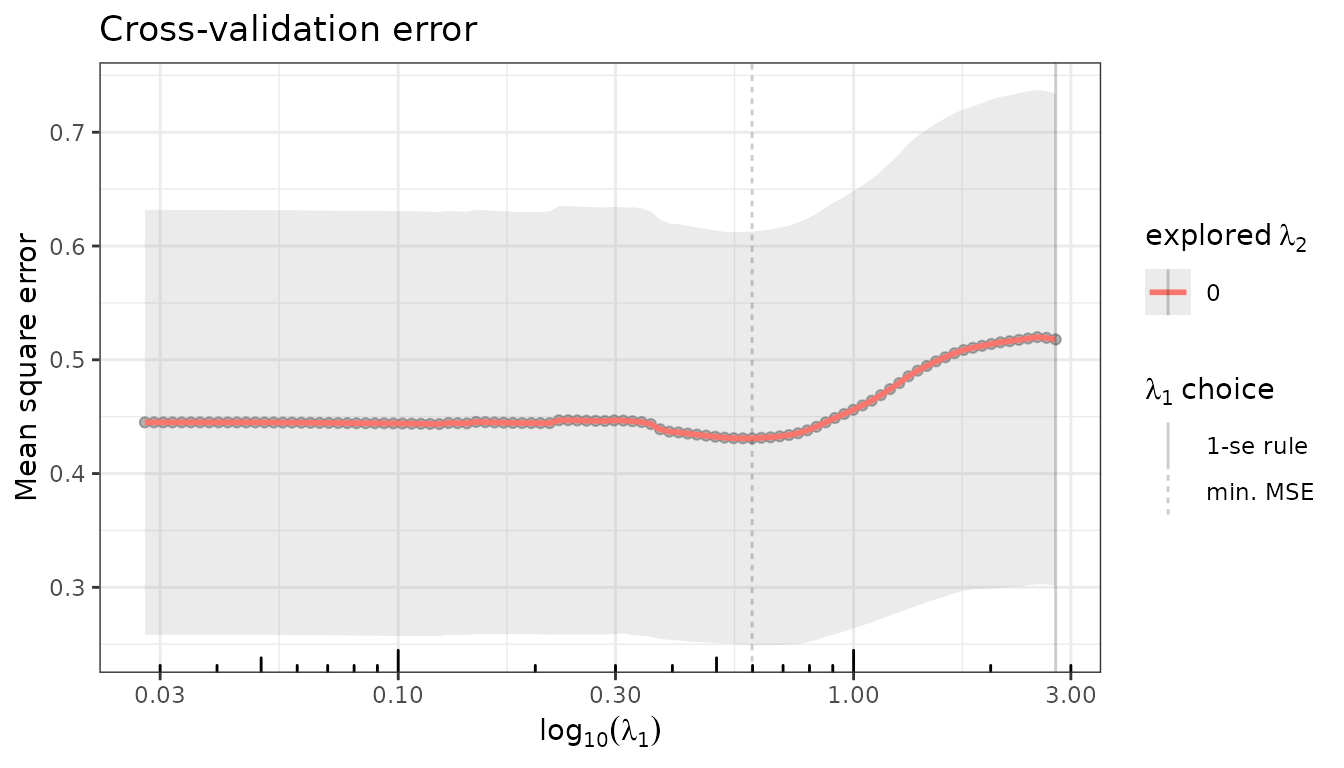
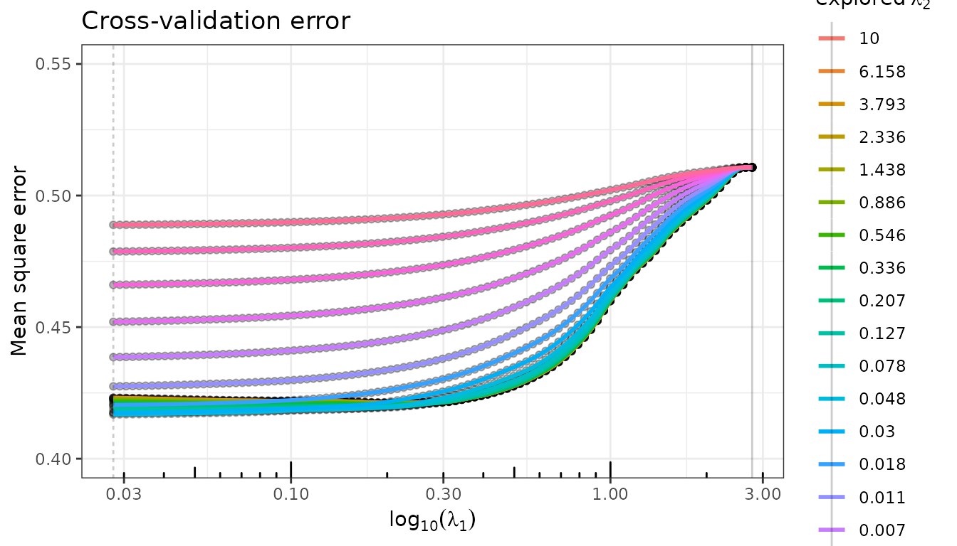
#>  0.05758491 -0.09951214

Cross-validation on $\lambda_1 \times \lambda_2$

For regularizers with two penalties (typically the Elastic-net), cross-validation can be run on a two-dimensional grid:

set.seed(42)
fit_enet$cross_validate(K = 5, lambda2 = 10^seq(1, -3, len=20), verbose = FALSE)

fit_enet$plot(type = "crossval")
fit_enet$cross_validation$plotCV_1D(se =  FALSE) + ggplot2::ylim(c(0.4, 0.55))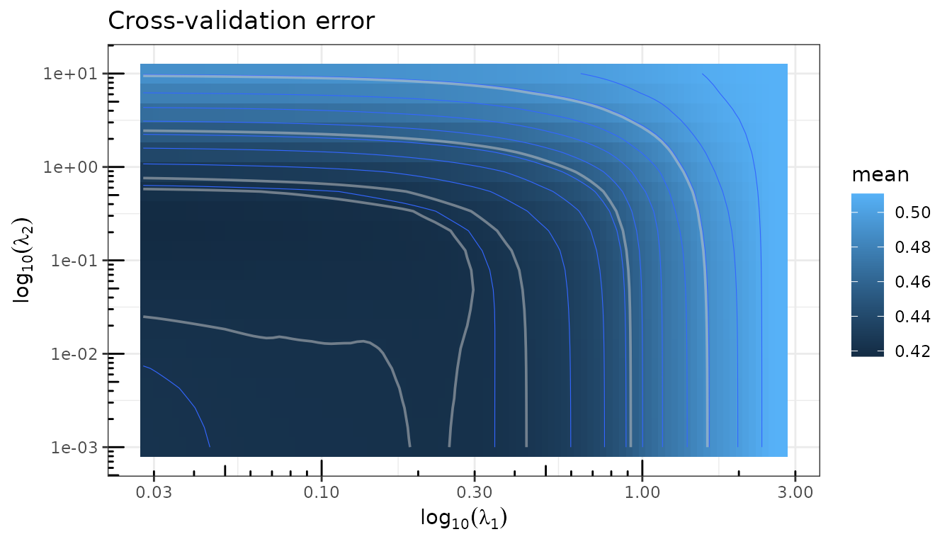

Prediction

$predict() returns fitted values for the whole path, or for a specific model selected by a criterion or a lambda value.

## Predictions at the CV_min-selected model
y_hat_lasso <- fit_lasso$predict(selection = "CV_min")
y_hat_mcp   <- fit_mcp$predict(selection = "CV_min")
y_hat_enet  <- fit_enet$predict(selection = "CV_min")

## R² at the selected model
r2_lasso <- fit_lasso$r_squared[fit_lasso$get_model("CV_min", type = "index")]
r2_mcp   <- fit_mcp$r_squared[fit_mcp$get_model("CV_min", type = "index")]
r2_enet  <- fit_enet$r_squared[fit_enet$get_model("CV_min", type = "index")]
cat(sprintf("R² Lasso (CV_min): %.3f\nR² MCP   (CV_min): %.3f\nR² Enet  (CV_min): %.3f\n", r2_lasso, r2_mcp, r2_enet))
#> R² Lasso (CV_min): 0.276
#> R² MCP   (CV_min): 0.265
#> R² Enet  (CV_min): 0.218

Stability selection

$stability() estimates selection probabilities via repeated sub-sampling (Meinshausen & Bühlmann, 2010). Variables that appear consistently across sub-samples receive high probabilities and are considered robustly selected. The stability path is stored as a [StabilityPath] R6 object in the field $stability_path of the current fit.

set.seed(42)
fit_lasso$stability(n_subsamples = 200, verbose = FALSE)

fit_lasso$plot(type = "stability")
#> Warning: This manual palette can handle a maximum of 13 values. You have
#> supplied 16
#> Warning: Removed 300 rows containing missing values or values outside the scale range
#> (`geom_line()`).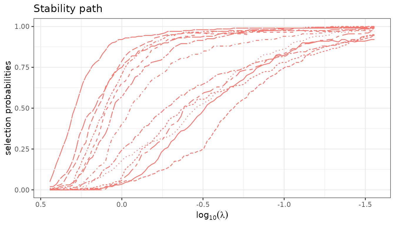

fit_lasso$stability_path$plot(nvarsel = 7)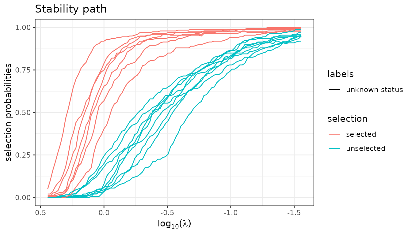

colnames(X)[fit_lasso$stability_path$selection(nvarsel = 7) ]
#> [1] "ui"    "white" "ptl1"  "smoke" "lwt1"  "ht"    "lwt3"

Debiased Estimators

Every $\ell_1$-based regularizer is known to be biased due to the shrinkage effect. A standard remedy is to refit the model on the selected support without penalization. This is implemented in quadrupen at no extra computational cost — the refitted coefficients are computed alongside the regularization path — and can be activated by setting the $debias field to TRUE.

fit_lasso$debias <- TRUE
fit_lasso$plot_path()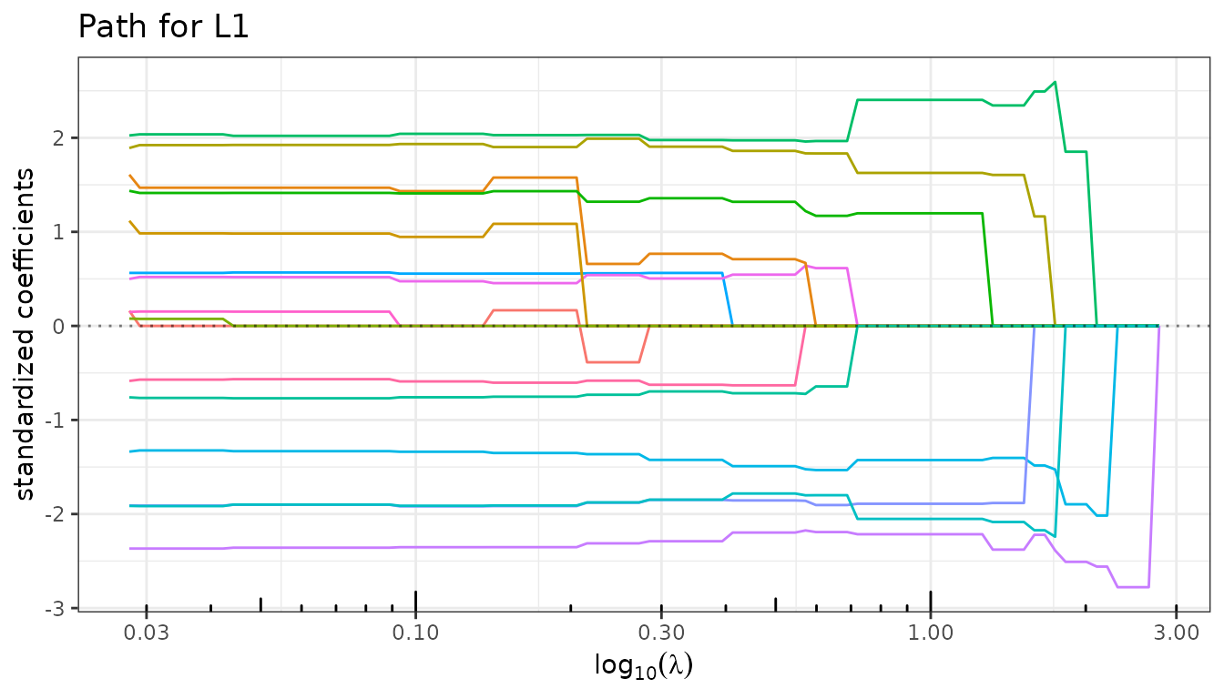

Since both versions are stored in the same object, it is straightforward to compare the regularized and debiased solutions — for the path as well as for CV error — by toggling $debias.

fit_lasso$cross_validate(verbose = FALSE)
fit_lasso$plot(type = "crossval")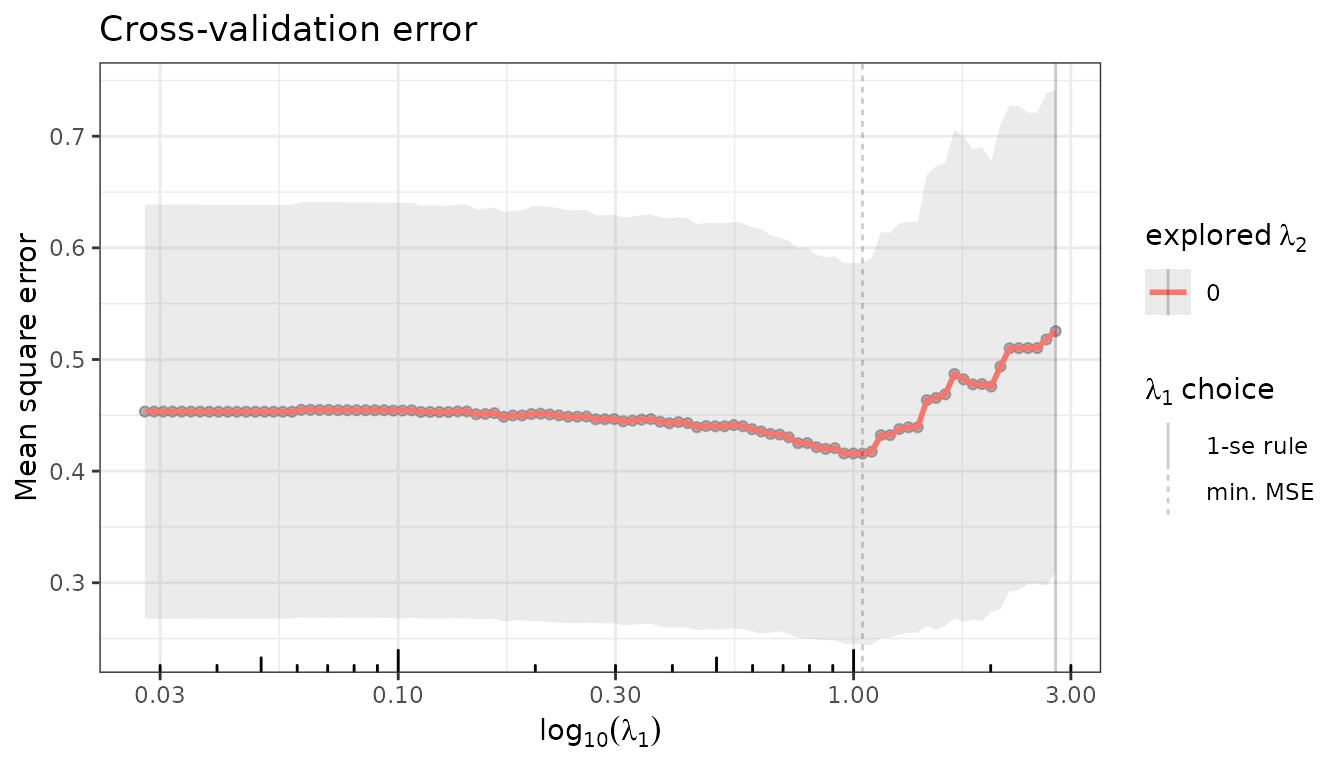

fit_lasso$debias <- FALSE
fit_lasso$plot_path()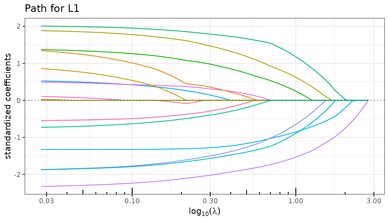

Setting $debias back to FALSE restores the original regularized coefficients.

A tour of standard analysis (fit, cross-validation, information criteria, stability)