Fit a linear model with a structured ridge regularization

Adjust a linear model with ridge regularization (possibly structured \(\ell_2\)-norm). The solution path is computed at a grid of values for the \(\ell_2\)-penalty. See details for the criterion optimized.

Usage

ridge(
  x,
  y,
  lambda = NULL,
  weights = rep(1, nrow(x)),
  struct = Matrix::Diagonal(ncol(x), 1),
  penscale = rep(1, ncol(x)),
  intercept = TRUE,
  normalize = TRUE,
  nlambda = 100,
  minratio = 1e-05,
  lambda_max = 100,
  control = list()
)

Arguments

x

matrix of features, possibly sparsely encoded (experimental). Do NOT include intercept. When normalized is TRUE, coefficients will then be rescaled to the original scale.

y

response vector.

lambda

sequence of decreasing \(\ell_2\)-penalty levels. If NULL (the default), a vector is generated with nlambda entries, starting from a guessed level lambda_max where only the intercept is included, then shrunken to minratio*lambda_max.

weights

vector with real positive values that weight the observations (like in weighted least square). Default sets all weights to 1.

struct

matrix structuring the coefficients, possibly sparsely encoded. Must be at least positive semidefinite (this is checked internally). If NULL (the default), the identity matrix is used. See details below.

penscale

vector with real positive values that weight the penalty of each feature. Default sets all weights to 1.

intercept

logical; indicates if an intercept should be included in the model. Default is TRUE.

normalize

logical; indicates if variables should be normalized to have unit L2 norm before fitting. Default is TRUE.

nlambda

integer that indicates the number of values to put in the lambda vector. Ignored if lambda is provided.

minratio

minimal value of \(\ell_1\)-part of the penalty that will be tried, as a fraction of the maximal lambda1 value. A too small value might lead to instability at the end of the solution path corresponding to small lambda1 combined with \(\lambda_2=0\). The default value tries to avoid this, adapting to the '\(n<p\)' context. Ignored if lambda1 is provided.

lambda_max

the largest value of lambda considered

control

list of argument controlling low level options of the algorithm –use with care and at your own risk– :

verbose: integer; activate verbose mode –this one is not too risky!– set to 0 for no output; 1 for warnings only, and 2 for tracing the whole progression. Default is 1. Automatically set to 0 when the method is embedded within cross-validation or stability selection.
timer: logical; use to record the timing of the algorithm. Default is FALSE.
maxiter the maximal number of iteration used in the active set algorithm to solve the problem for a given value of lambda1 . Default is 50.
method a string for the underlying solver used. Either "quadra", "fista" or "pgd". Default is "quadra".
factmat Boolean indicating if matrix factorization should be used to solve the sub-system. If TRUE (the default), a Cholesky decomposition is maintained along the path. If FALSE, the sub-system are solved with a conjugate gradient algorithm.
threshold a threshold for convergence. The algorithm stops when the optimality conditions are fulfill up to this threshold. Default is 1e-6.
monitor indicates if a monitoring of the convergence should be recorded, by computing a lower bound between the current solution and the optimum: when '0' (the default), no monitoring is provided; when '1', the bound derived in Grandvalet et al. is computed; when '>1', the Fenchel duality gap is computed along the algorithm.

Value

an object with class RidgeRegressionFit, inheriting from QuadrupenFit.

Details

The optimized criterion is the following: β^hat_λ₂ = argmin_β 1/2 RSS(β) + λ/2 ₂ β^T S β, where the \(\ell_2\) structuring positive semidefinite matrix \(S\) is provided via the struct argument (possibly of class Matrix).

Examples

## Simulating multivariate Gaussian with blockwise correlation
## and piecewise constant vector of parameters
beta <- rep(c(0,1,0,-1,0), c(25,10,25,10,25))
cor <- 0.75
Soo <- toeplitz(cor^(0:(25-1))) ## Toeplitz correlation for irrelevant variables
Sww  <- matrix(cor,10,10) ## bloc correlation between active variables
Sigma <- Matrix::bdiag(Soo,Sww,Soo,Sww,Soo)
diag(Sigma) <- 1
n <- 50
x <- as.matrix(matrix(rnorm(95*n),n,95) %*% chol(Sigma))
y <- 10 + x %*% beta + rnorm(n,0,10)

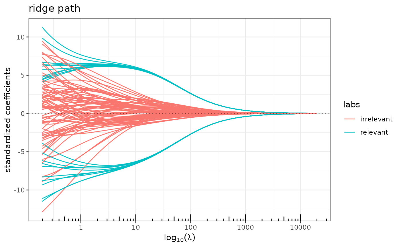
labels <- rep("irrelevant", length(beta))
labels[beta != 0] <- "relevant"
plot(ridge(x,y) , label=labels) ## a mess

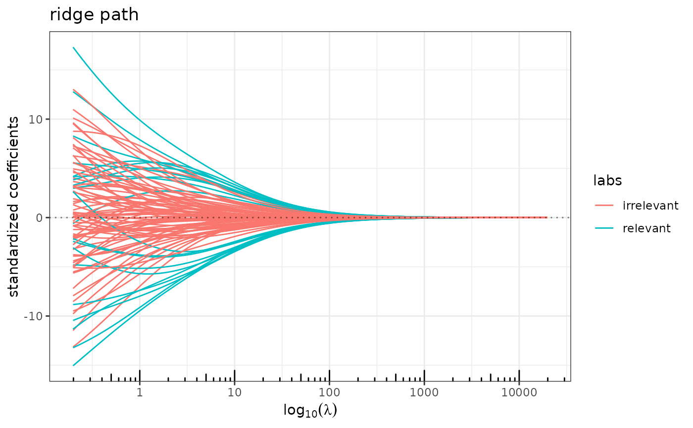plot(ridge(x,y, struct=solve(Sigma)), label=labels) ## even better