Homework: PCA

PCA for visualization, compression and exploratory analyses

Information

Data sets are available at https://github.com/jchiquet/MAP573/tree/master/data. Homework is due Sunday 10/18 23:59 in Rmd (see assignment in Moodle).

Package requirements

We start by loading a couple of packages for data manipulation, dimension reduction and fancy representations.

library(tidyverse)    # advanced data manipulation and vizualisation
library(knitr)        # R notebook export and formatting 
library(FactoMineR)   # Factor analysis
library(factoextra)   # Fancy plotting of FactoMineR outputs
library(kableExtra)   # integration of table in Rmarkdown
theme_set(theme_bw()) # set default ggplot2 theme to black and white

SNP data: genotyping of various population

Data description

A single-nucleotide polymorphism is a substitution of a single nucleotide that occurs at a specific position in the genome, where each variation is present at a level of 0.5% from person to person in the population. They are coded as 0, 1 or 2 (meaning 0, 1 or 2 allels different regarding the reference population)

See the great wikipedia page for detail!

We can measure SNP for individuals with high trhoughput technology and SNP array. SNP chips for human contains more than 1 million variables! We only suggest to analyse a sample of a data set containing the 5500 most variant SNP for 728 individuals with various origin, with the following descriptors:

• CEU: Utah residents with Northern and Western European ancestry from the CEPH collection
• GIH: Gujarati Indians in Houston, Texas
• LWK: Luhya in Webuye, Kenya
• MKK: Maasai in Kinyawa, Kenya
• TSI: Toscani in Italia
• YRI: Yoruba in Ibadan, Nigeria

The data are imported as follows:

load("data/SNP.RData")
snp  <- data$Geno %>% as_tibble() %>%
  add_column(origin = data$origin, .before = 1) 

Questions

0. Have a look at the data a make some brief descriptive plot/summary
1. Fit a PCA on these data. Justify the scaling or not.
2. Represent the scree plot for the 100 first axes. Comment. Estimate the number of axis with estim_npc
3. Plot individual factor maps on axes 1, 2 and 3. Add colors and ellipses associated with the factor ‘origin’
4. Check who are the first, say, 250 most contributive individuals to these axes. Show them in the projection. Have a look at the cosine of the most influent guys.
5. Plot the correlation circle. Only retain variables based on the quality of their representation and/or degree of contribution to the axes represented.
6. Summarize the above analyses in biplots. Add fancy colors and whatever.
7. Indicate a group of individual as supplementary (i.e., not use to fit the PC). Show how excluding a group influence (or not) the fit and the projection, by exploring several groups. Explain.

Solution

0. Have a look at the data a make some brief descriptive plot/summary

The first column is a categorical variable describing the orgin of each individual, with details on the acronyme given above

barplot(table(snp$origin), las = 3, main = 'distribution of origin')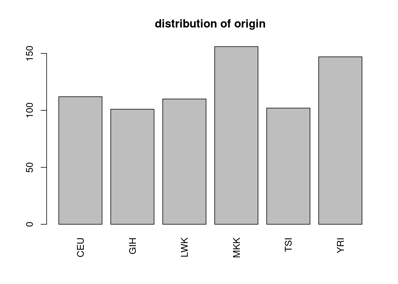

1. Fit a PCA on these data. Justify the scaling or not.

I do not scale, since SNP value are suppose to live on the same scale (values in \(\{0, 1, 2\}\)).

acp <- PCA(snp, quali.sup = 1, scale.unit = FALSE, graph = FALSE, ncp = 500)

## Warning in PCA(snp, quali.sup = 1, scale.unit = FALSE, graph = FALSE, ncp =
## 500): Missing values are imputed by the mean of the variable: you should use the
## imputePCA function of the missMDA package

2. Represent the scree plot for the 100 first axes. Comment

First axes are more informative than the other, and then the information is generally well spread.

fviz_eig(acp, ncp = 100)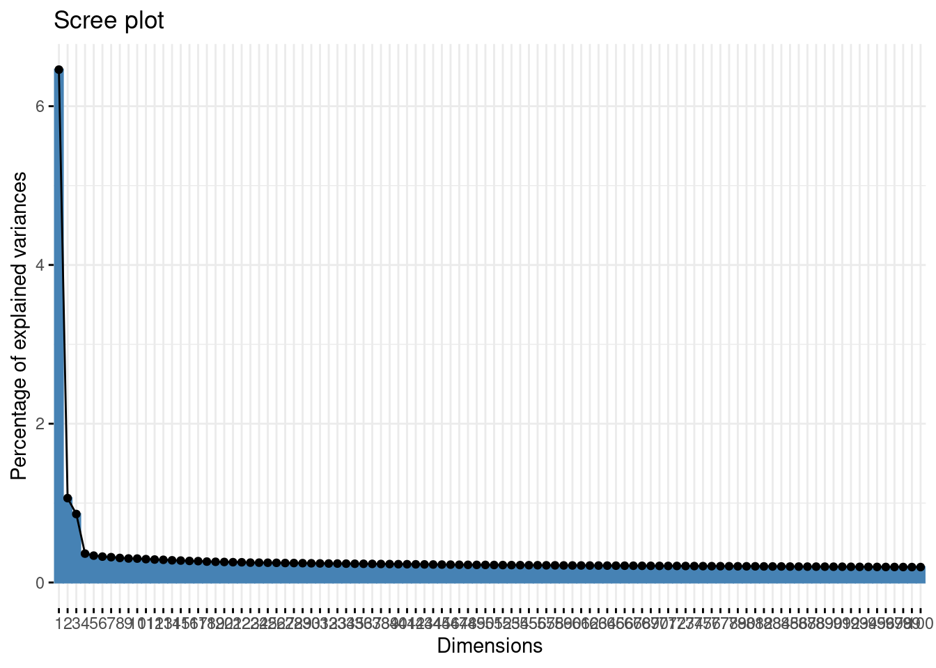

npc <- select(snp, -origin) %>% replace(is.na(.), 0) %>% 
    as.matrix() %>% scale(TRUE, FALSE) %>% 
    estim_ncp(ncp.max = 15, scale = FALSE) 
plot(npc$criterion, type = "b", xlab = 'number of component', ylab = 'GCV')

3. Plot individual factor maps on axes 1, 2 and 3. Add color and ellipse associated with the origin

Argument habillage or col.ind will have the same effect, but the first will be more useful later.

Impressive how the population are well separated!

fviz_pca_ind(acp, habillage = "origin", addEllipses = TRUE)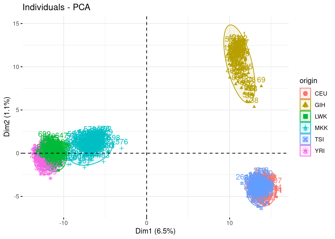

fviz_pca_ind(acp, habillage =  "origin", axes = c(1,3), addEllipses = TRUE)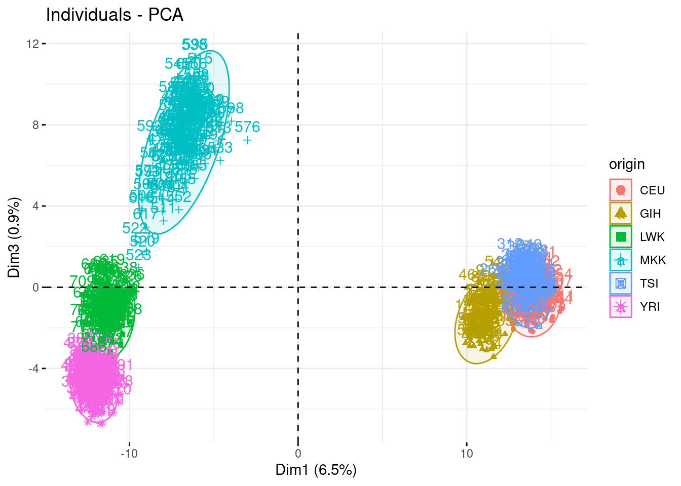

fviz_pca_ind(acp, habillage = "origin", axes = c(2,3), addEllipses = TRUE)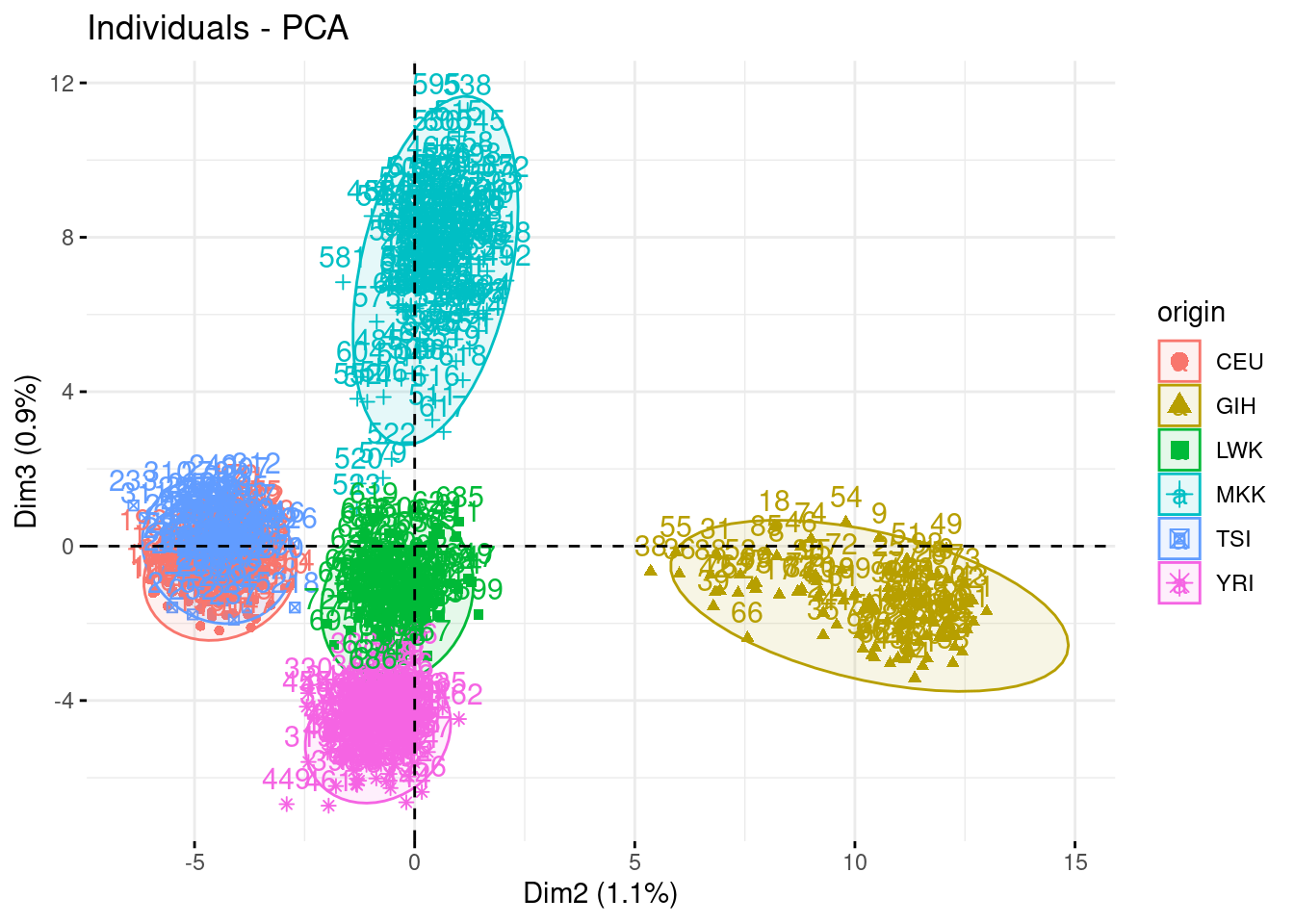

4. Check who are the first, say, 250 most contributive individual to these axes. Show them in the projection. Have a look at the cosine of the most influent guys.

fviz_contrib(acp, "ind", axes = 1:3, top = 250)

fviz_pca_ind(acp, habillage = "origin", select.ind = list(contrib = 250))

fviz_pca_ind(acp, axes = c(2,3),  habillage = "origin", select.ind = list(contrib = 250))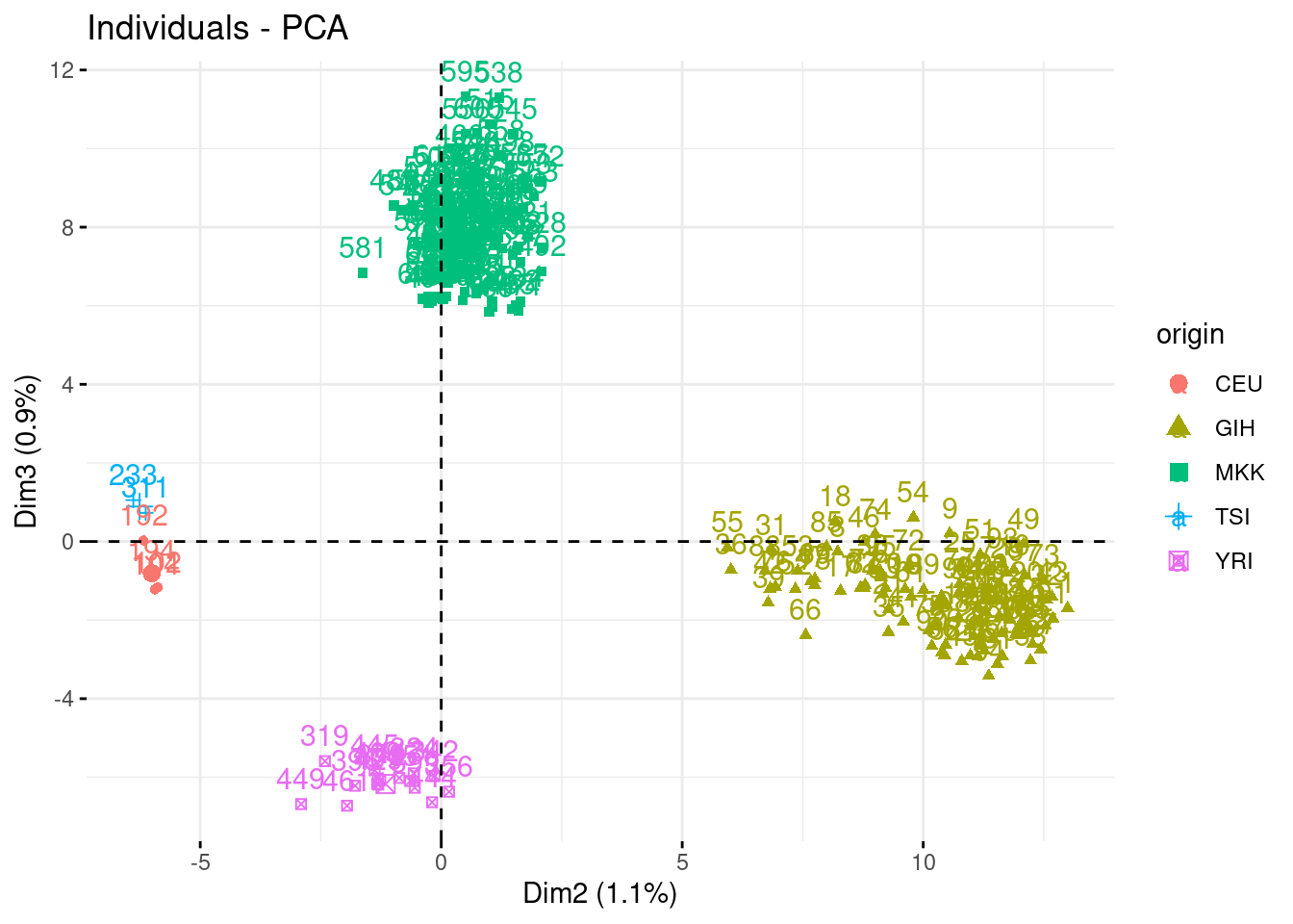

fviz_pca_ind(acp, habillage = "origin", select.ind = list(contrib = 250))

fviz_pca_ind(acp, habillage = "origin", select.ind = list(contrib = 250))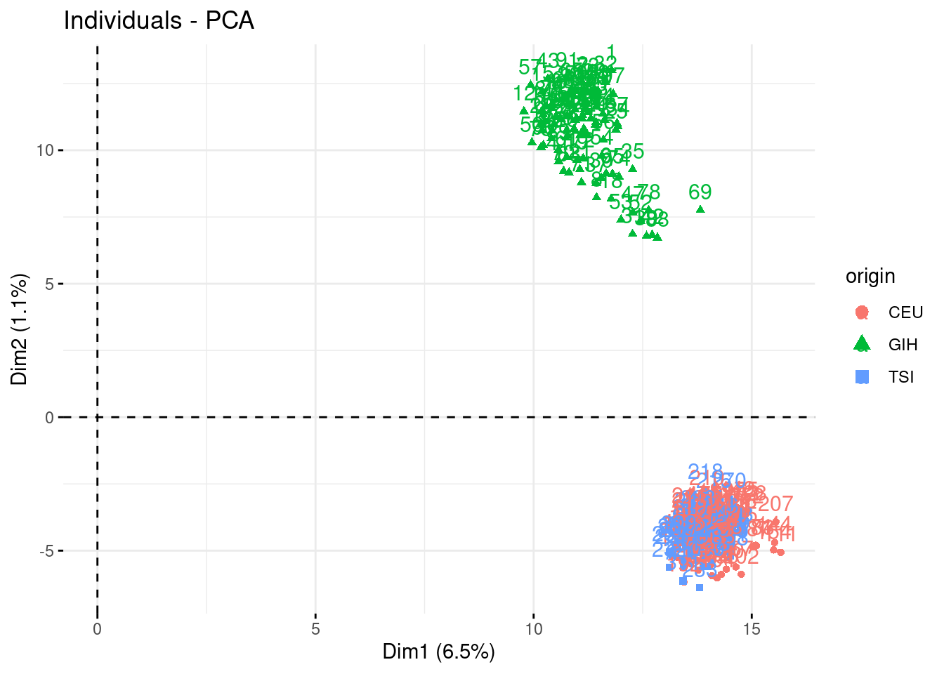

5. Plot the correlation circle. Only retain variables based on the quality of their representation and/or degree of contribution to the axes represented.

fviz_contrib(acp, "var", axes = 1:3, top = 500)

fviz_pca_var(acp, select.var = list(contrib = 50), col.var = 'cos2')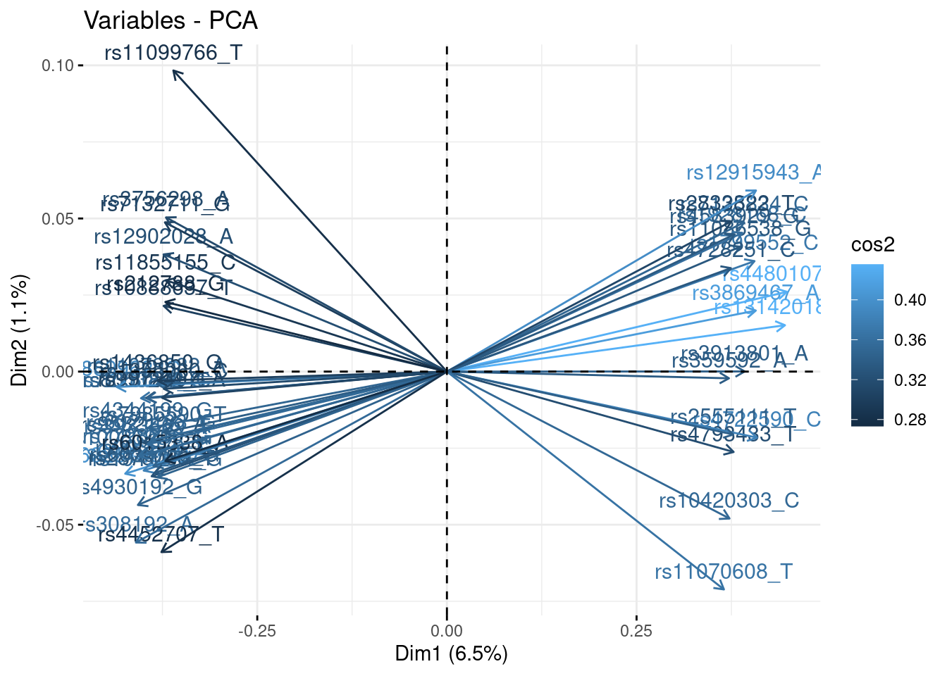

6. Summarize the above analyses in biplots. Add fancy colors

Just example, you can do better/different than that!

fviz_pca_biplot(acp, axes = c(1,3), habillage = "origin", addEllipses = TRUE, select.var = list(contrib = 40))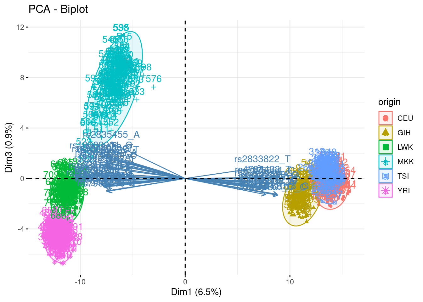

fviz_pca_biplot(acp, axes = c(1,3), habillage = "origin", addEllipses = TRUE, select.var = list(contrib = 40))

fviz_pca_biplot(acp, axes = c(2,3), habillage = "origin", addEllipses = TRUE, select.var = list(contrib = 40))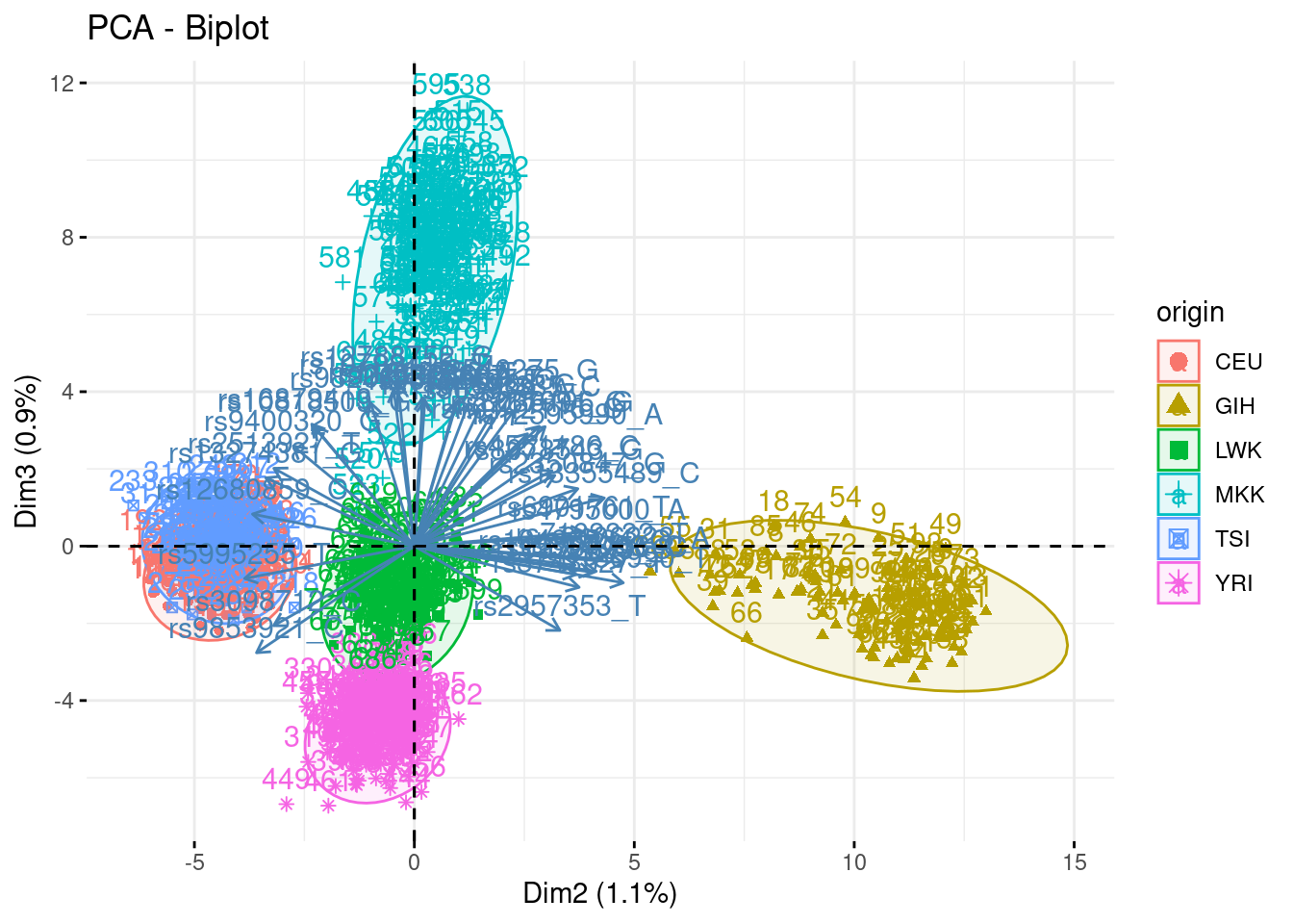

7. Indicate a group of individual as supplmentary (i.e., not use to fit the PC). Show how excluding a group influence (or not) the fit and the projection, by exploring several groups. Explain

Depending on the proximity of the group to the cloud and to some particular existing groups, the fit is more or less altered.

acp_noMKK <- PCA(snp, quali.sup = 1, ind.sup = which(snp$origin == "MKK"), scale.unit = FALSE, graph = FALSE, ncp = 500)

## Warning in PCA(snp, quali.sup = 1, ind.sup = which(snp$origin == "MKK"), :
## Missing values are imputed by the mean of the variable: you should use the
## imputePCA function of the missMDA package

fviz_pca_biplot(acp, habillage = "origin", addEllipses = TRUE, select.var = list(contrib = 40), col.ind.sup = "black")

acp_noTSI <- PCA(snp, quali.sup = 1, ind.sup = which(snp$origin == "TSI"), scale.unit = FALSE, graph = FALSE, ncp = 500)

## Warning in PCA(snp, quali.sup = 1, ind.sup = which(snp$origin == "TSI"), :
## Missing values are imputed by the mean of the variable: you should use the
## imputePCA function of the missMDA package

fviz_pca_biplot(acp, habillage = "origin", addEllipses = TRUE, select.var = list(contrib = 40), col.ind.sup = "black")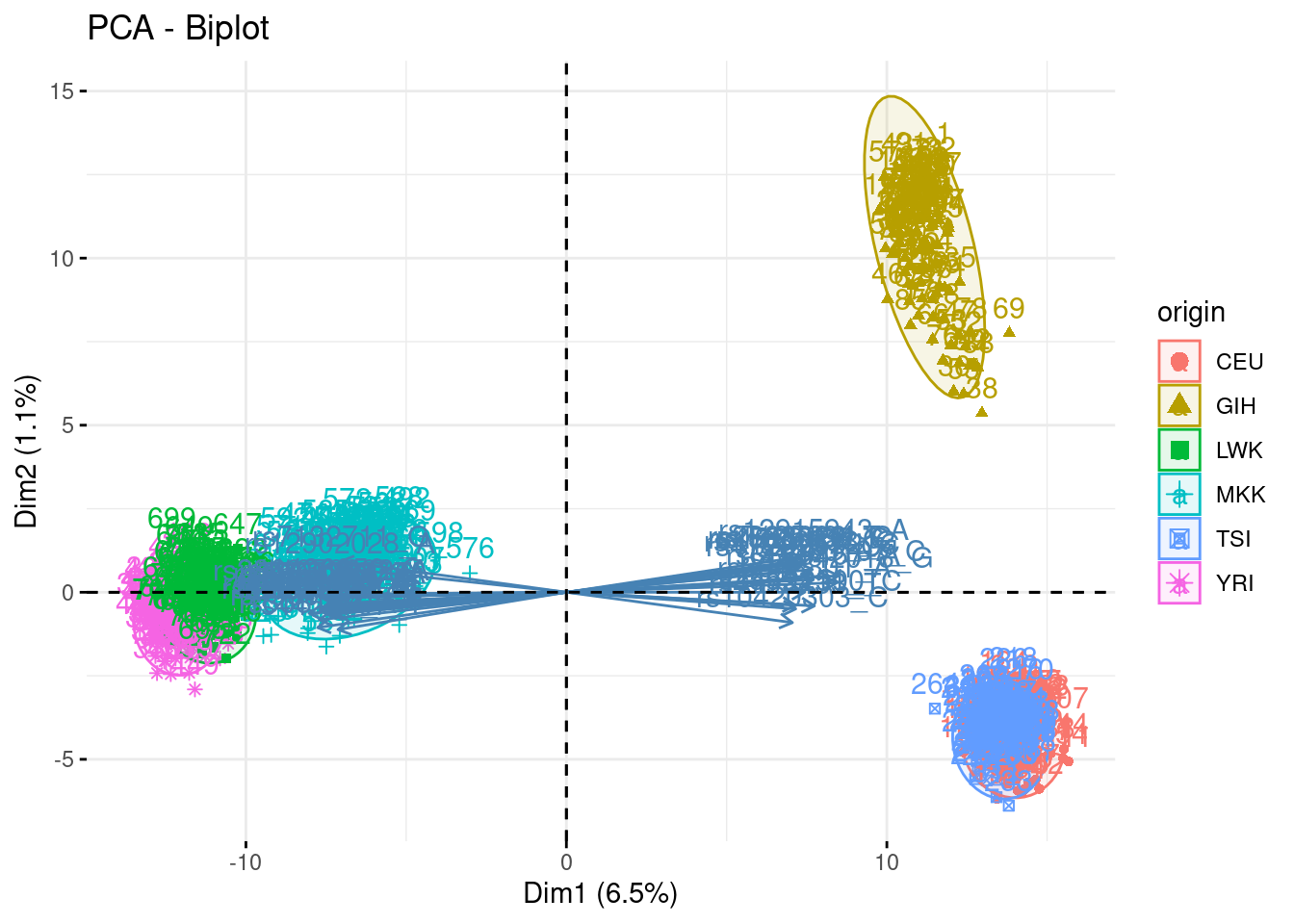

acp_noGIH <- PCA(snp, quali.sup = 1, ind.sup = which(snp$origin == "GIH"), scale.unit = FALSE, graph = FALSE, ncp = 500)

## Warning in PCA(snp, quali.sup = 1, ind.sup = which(snp$origin == "GIH"), :
## Missing values are imputed by the mean of the variable: you should use the
## imputePCA function of the missMDA package

fviz_pca_biplot(acp, habillage = "origin", addEllipses = TRUE, select.var = list(contrib = 25), col.ind.sup = "black")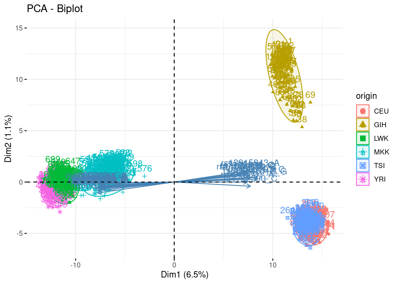

fviz_pca_biplot(acp, axes = c(2,3), habillage = "origin", addEllipses = TRUE, select.var = list(contrib = 25), col.ind.sup = "black")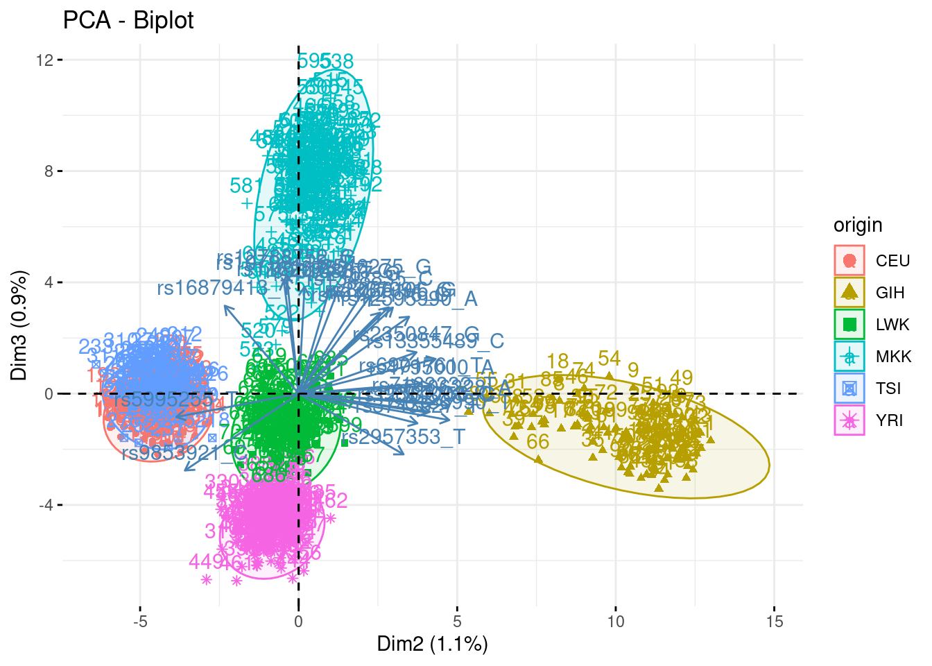

MNIST data: handwritten digit data

Data description

The MNIST dataset is an acronym that stands for the Modified National Institute of Standards and Technology dataset. It is a dataset of 60,000 small square 28×28 pixel grayscale images of handwritten single digits between 0 and 9. It is commonly used for training various image processing systems. The database is also widely used for training and testing in the field of machine learning.

The full data set is available here.

But careful!!, it weigths more than 100 Mo so check your internet connection

A sample of 2,000 instances is provided for convenience mnist_sample.

Questions

1. Load an format the data (first column is the label) as a tibble or a data.frame. Each row is a vector with size 784 (28 x 28) + a column for the label.
2. Write a function to plot an 28 x 28 image based on a vector, and test it on a row of your data frame.
3. Make a PCA, choice whether to scale or not.
4. Make the usual diagnostic plots (screeplot, individual, variable) for the first axes, and comment. Use GCV to select the number of axes.
5. Write a function to reconstruct an image with two argument: \(i\) (an instance) \(k\) (the number of component used).
6. Plot the reconstructed image for various value of \(k\)

Solution

1. Load an format the data (first column is the label) as a tibble or a data.frame. Each row is a vector with size 784 (28 x 28) + a column for the label.

mnist_raw <- read_csv("data/mnist_sample.csv", col_names = FALSE, n_max = 2000)

mnist <- mnist_raw %>%
  rename(label = X1) %>%
  mutate(instance = row_number())
mnist %>% head() %>% kable() %>% kable_styling() %>%
  scroll_box(width = "100%")

label	X2	X3	X4	X5	X6	X7	X8	X9	X10	X11	X12	X13	X14	X15	X16	X17	X18	X19	X20	X21	X22	X23	X24	X25	X26	X27	X28	X29	X30	X31	X32	X33	X34	X35	X36	X37	X38	X39	X40	X41	X42	X43	X44	X45	X46	X47	X48	X49	X50	X51	X52	X53	X54	X55	X56	X57	X58	X59	X60	X61	X62	X63	X64	X65	X66	X67	X68	X69	X70	X71	X72	X73	X74	X75	X76	X77	X78	X79	X80	X81	X82	X83	X84	X85	X86	X87	X88	X89	X90	X91	X92	X93	X94	X95	X96	X97	X98	X99	X100	X101	X102	X103	X104	X105	X106	X107	X108	X109	X110	X111	X112	X113	X114	X115	X116	X117	X118	X119	X120	X121	X122	X123	X124	X125	X126	X127	X128	X129	X130	X131	X132	X133	X134	X135	X136	X137	X138	X139	X140	X141	X142	X143	X144	X145	X146	X147	X148	X149	X150	X151	X152	X153	X154	X155	X156	X157	X158	X159	X160	X161	X162	X163	X164	X165	X166	X167	X168	X169	X170	X171	X172	X173	X174	X175	X176	X177	X178	X179	X180	X181	X182	X183	X184	X185	X186	X187	X188	X189	X190	X191	X192	X193	X194	X195	X196	X197	X198	X199	X200	X201	X202	X203	X204	X205	X206	X207	X208	X209	X210	X211	X212	X213	X214	X215	X216	X217	X218	X219	X220	X221	X222	X223	X224	X225	X226	X227	X228	X229	X230	X231	X232	X233	X234	X235	X236	X237	X238	X239	X240	X241	X242	X243	X244	X245	X246	X247	X248	X249	X250	X251	X252	X253	X254	X255	X256	X257	X258	X259	X260	X261	X262	X263	X264	X265	X266	X267	X268	X269	X270	X271	X272	X273	X274	X275	X276	X277	X278	X279	X280	X281	X282	X283	X284	X285	X286	X287	X288	X289	X290	X291	X292	X293	X294	X295	X296	X297	X298	X299	X300	X301	X302	X303	X304	X305	X306	X307	X308	X309	X310	X311	X312	X313	X314	X315	X316	X317	X318	X319	X320	X321	X322	X323	X324	X325	X326	X327	X328	X329	X330	X331	X332	X333	X334	X335	X336	X337	X338	X339	X340	X341	X342	X343	X344	X345	X346	X347	X348	X349	X350	X351	X352	X353	X354	X355	X356	X357	X358	X359	X360	X361	X362	X363	X364	X365	X366	X367	X368	X369	X370	X371	X372	X373	X374	X375	X376	X377	X378	X379	X380	X381	X382	X383	X384	X385	X386	X387	X388	X389	X390	X391	X392	X393	X394	X395	X396	X397	X398	X399	X400	X401	X402	X403	X404	X405	X406	X407	X408	X409	X410	X411	X412	X413	X414	X415	X416	X417	X418	X419	X420	X421	X422	X423	X424	X425	X426	X427	X428	X429	X430	X431	X432	X433	X434	X435	X436	X437	X438	X439	X440	X441	X442	X443	X444	X445	X446	X447	X448	X449	X450	X451	X452	X453	X454	X455	X456	X457	X458	X459	X460	X461	X462	X463	X464	X465	X466	X467	X468	X469	X470	X471	X472	X473	X474	X475	X476	X477	X478	X479	X480	X481	X482	X483	X484	X485	X486	X487	X488	X489	X490	X491	X492	X493	X494	X495	X496	X497	X498	X499	X500	X501	X502	X503	X504	X505	X506	X507	X508	X509	X510	X511	X512	X513	X514	X515	X516	X517	X518	X519	X520	X521	X522	X523	X524	X525	X526	X527	X528	X529	X530	X531	X532	X533	X534	X535	X536	X537	X538	X539	X540	X541	X542	X543	X544	X545	X546	X547	X548	X549	X550	X551	X552	X553	X554	X555	X556	X557	X558	X559	X560	X561	X562	X563	X564	X565	X566	X567	X568	X569	X570	X571	X572	X573	X574	X575	X576	X577	X578	X579	X580	X581	X582	X583	X584	X585	X586	X587	X588	X589	X590	X591	X592	X593	X594	X595	X596	X597	X598	X599	X600	X601	X602	X603	X604	X605	X606	X607	X608	X609	X610	X611	X612	X613	X614	X615	X616	X617	X618	X619	X620	X621	X622	X623	X624	X625	X626	X627	X628	X629	X630	X631	X632	X633	X634	X635	X636	X637	X638	X639	X640	X641	X642	X643	X644	X645	X646	X647	X648	X649	X650	X651	X652	X653	X654	X655	X656	X657	X658	X659	X660	X661	X662	X663	X664	X665	X666	X667	X668	X669	X670	X671	X672	X673	X674	X675	X676	X677	X678	X679	X680	X681	X682	X683	X684	X685	X686	X687	X688	X689	X690	X691	X692	X693	X694	X695	X696	X697	X698	X699	X700	X701	X702	X703	X704	X705	X706	X707	X708	X709	X710	X711	X712	X713	X714	X715	X716	X717	X718	X719	X720	X721	X722	X723	X724	X725	X726	X727	X728	X729	X730	X731	X732	X733	X734	X735	X736	X737	X738	X739	X740	X741	X742	X743	X744	X745	X746	X747	X748	X749	X750	X751	X752	X753	X754	X755	X756	X757	X758	X759	X760	X761	X762	X763	X764	X765	X766	X767	X768	X769	X770	X771	X772	X773	X774	X775	X776	X777	X778	X779	X780	X781	X782	X783	X784	X785	instance
5	0	0	0	0	0	0	0	0	0	0	0	0	0	0	0	0	0	0	0	0	0	0	0	0	0	0	0	0	0	0	0	0	0	0	0	0	0	0	0	0	0	0	0	0	0	0	0	0	0	0	0	0	0	0	0	0	0	0	0	0	0	0	0	0	0	0	0	0	0	0	0	0	0	0	0	0	0	0	0	0	0	0	0	0	0	0	0	0	0	0	0	0	0	0	0	0	0	0	0	0	0	0	0	0	0	0	0	0	0	0	0	0	0	0	0	0	0	0	0	0	0	0	0	0	0	0	0	0	0	0	0	0	0	0	0	0	0	0	0	0	0	0	0	0	0	0	0	0	0	0	0	0	3	18	18	18	126	136	175	26	166	255	247	127	0	0	0	0	0	0	0	0	0	0	0	0	30	36	94	154	170	253	253	253	253	253	225	172	253	242	195	64	0	0	0	0	0	0	0	0	0	0	0	49	238	253	253	253	253	253	253	253	253	251	93	82	82	56	39	0	0	0	0	0	0	0	0	0	0	0	0	18	219	253	253	253	253	253	198	182	247	241	0	0	0	0	0	0	0	0	0	0	0	0	0	0	0	0	0	0	80	156	107	253	253	205	11	0	43	154	0	0	0	0	0	0	0	0	0	0	0	0	0	0	0	0	0	0	0	14	1	154	253	90	0	0	0	0	0	0	0	0	0	0	0	0	0	0	0	0	0	0	0	0	0	0	0	0	0	139	253	190	2	0	0	0	0	0	0	0	0	0	0	0	0	0	0	0	0	0	0	0	0	0	0	0	0	11	190	253	70	0	0	0	0	0	0	0	0	0	0	0	0	0	0	0	0	0	0	0	0	0	0	0	0	0	35	241	225	160	108	1	0	0	0	0	0	0	0	0	0	0	0	0	0	0	0	0	0	0	0	0	0	0	0	81	240	253	253	119	25	0	0	0	0	0	0	0	0	0	0	0	0	0	0	0	0	0	0	0	0	0	0	0	45	186	253	253	150	27	0	0	0	0	0	0	0	0	0	0	0	0	0	0	0	0	0	0	0	0	0	0	0	16	93	252	253	187	0	0	0	0	0	0	0	0	0	0	0	0	0	0	0	0	0	0	0	0	0	0	0	0	0	249	253	249	64	0	0	0	0	0	0	0	0	0	0	0	0	0	0	0	0	0	0	0	0	0	46	130	183	253	253	207	2	0	0	0	0	0	0	0	0	0	0	0	0	0	0	0	0	0	0	0	39	148	229	253	253	253	250	182	0	0	0	0	0	0	0	0	0	0	0	0	0	0	0	0	0	0	24	114	221	253	253	253	253	201	78	0	0	0	0	0	0	0	0	0	0	0	0	0	0	0	0	0	23	66	213	253	253	253	253	198	81	2	0	0	0	0	0	0	0	0	0	0	0	0	0	0	0	0	18	171	219	253	253	253	253	195	80	9	0	0	0	0	0	0	0	0	0	0	0	0	0	0	0	0	55	172	226	253	253	253	253	244	133	11	0	0	0	0	0	0	0	0	0	0	0	0	0	0	0	0	0	0	136	253	253	253	212	135	132	16	0	0	0	0	0	0	0	0	0	0	0	0	0	0	0	0	0	0	0	0	0	0	0	0	0	0	0	0	0	0	0	0	0	0	0	0	0	0	0	0	0	0	0	0	0	0	0	0	0	0	0	0	0	0	0	0	0	0	0	0	0	0	0	0	0	0	0	0	0	0	0	0	0	0	0	0	0	0	0	0	0	0	0	0	0	0	0	0	0	0	0	0	0	0	0	0	0	0	0	0	1
0	0	0	0	0	0	0	0	0	0	0	0	0	0	0	0	0	0	0	0	0	0	0	0	0	0	0	0	0	0	0	0	0	0	0	0	0	0	0	0	0	0	0	0	0	0	0	0	0	0	0	0	0	0	0	0	0	0	0	0	0	0	0	0	0	0	0	0	0	0	0	0	0	0	0	0	0	0	0	0	0	0	0	0	0	0	0	0	0	0	0	0	0	0	0	0	0	0	0	0	0	0	0	0	0	0	0	0	0	0	0	0	0	0	0	0	0	0	0	0	0	0	0	0	0	0	0	0	51	159	253	159	50	0	0	0	0	0	0	0	0	0	0	0	0	0	0	0	0	0	0	0	0	0	0	48	238	252	252	252	237	0	0	0	0	0	0	0	0	0	0	0	0	0	0	0	0	0	0	0	0	0	54	227	253	252	239	233	252	57	6	0	0	0	0	0	0	0	0	0	0	0	0	0	0	0	0	0	10	60	224	252	253	252	202	84	252	253	122	0	0	0	0	0	0	0	0	0	0	0	0	0	0	0	0	0	163	252	252	252	253	252	252	96	189	253	167	0	0	0	0	0	0	0	0	0	0	0	0	0	0	0	0	51	238	253	253	190	114	253	228	47	79	255	168	0	0	0	0	0	0	0	0	0	0	0	0	0	0	0	48	238	252	252	179	12	75	121	21	0	0	253	243	50	0	0	0	0	0	0	0	0	0	0	0	0	0	38	165	253	233	208	84	0	0	0	0	0	0	253	252	165	0	0	0	0	0	0	0	0	0	0	0	0	7	178	252	240	71	19	28	0	0	0	0	0	0	253	252	195	0	0	0	0	0	0	0	0	0	0	0	0	57	252	252	63	0	0	0	0	0	0	0	0	0	253	252	195	0	0	0	0	0	0	0	0	0	0	0	0	198	253	190	0	0	0	0	0	0	0	0	0	0	255	253	196	0	0	0	0	0	0	0	0	0	0	0	76	246	252	112	0	0	0	0	0	0	0	0	0	0	253	252	148	0	0	0	0	0	0	0	0	0	0	0	85	252	230	25	0	0	0	0	0	0	0	0	7	135	253	186	12	0	0	0	0	0	0	0	0	0	0	0	85	252	223	0	0	0	0	0	0	0	0	7	131	252	225	71	0	0	0	0	0	0	0	0	0	0	0	0	85	252	145	0	0	0	0	0	0	0	48	165	252	173	0	0	0	0	0	0	0	0	0	0	0	0	0	0	86	253	225	0	0	0	0	0	0	114	238	253	162	0	0	0	0	0	0	0	0	0	0	0	0	0	0	0	85	252	249	146	48	29	85	178	225	253	223	167	56	0	0	0	0	0	0	0	0	0	0	0	0	0	0	0	85	252	252	252	229	215	252	252	252	196	130	0	0	0	0	0	0	0	0	0	0	0	0	0	0	0	0	0	28	199	252	252	253	252	252	233	145	0	0	0	0	0	0	0	0	0	0	0	0	0	0	0	0	0	0	0	0	25	128	252	253	252	141	37	0	0	0	0	0	0	0	0	0	0	0	0	0	0	0	0	0	0	0	0	0	0	0	0	0	0	0	0	0	0	0	0	0	0	0	0	0	0	0	0	0	0	0	0	0	0	0	0	0	0	0	0	0	0	0	0	0	0	0	0	0	0	0	0	0	0	0	0	0	0	0	0	0	0	0	0	0	0	0	0	0	0	0	0	0	0	0	0	0	0	0	0	0	0	0	0	0	0	0	0	0	0	0	0	0	0	0	0	0	0	0	0	0	0	0	0	0	0	0	0	0	0	0	0	0	0	2
4	0	0	0	0	0	0	0	0	0	0	0	0	0	0	0	0	0	0	0	0	0	0	0	0	0	0	0	0	0	0	0	0	0	0	0	0	0	0	0	0	0	0	0	0	0	0	0	0	0	0	0	0	0	0	0	0	0	0	0	0	0	0	0	0	0	0	0	0	0	0	0	0	0	0	0	0	0	0	0	0	0	0	0	0	0	0	0	0	0	0	0	0	0	0	0	0	0	0	0	0	0	0	0	0	0	0	0	0	0	0	0	0	0	0	0	0	0	0	0	0	0	0	0	0	0	0	0	0	0	0	0	0	0	0	0	0	0	0	0	0	0	0	0	0	0	0	0	0	0	0	0	0	0	0	0	0	0	0	0	0	67	232	39	0	0	0	0	0	0	0	0	0	62	81	0	0	0	0	0	0	0	0	0	0	0	0	0	0	120	180	39	0	0	0	0	0	0	0	0	0	126	163	0	0	0	0	0	0	0	0	0	0	0	0	0	2	153	210	40	0	0	0	0	0	0	0	0	0	220	163	0	0	0	0	0	0	0	0	0	0	0	0	0	27	254	162	0	0	0	0	0	0	0	0	0	0	222	163	0	0	0	0	0	0	0	0	0	0	0	0	0	183	254	125	0	0	0	0	0	0	0	0	0	46	245	163	0	0	0	0	0	0	0	0	0	0	0	0	0	198	254	56	0	0	0	0	0	0	0	0	0	120	254	163	0	0	0	0	0	0	0	0	0	0	0	0	23	231	254	29	0	0	0	0	0	0	0	0	0	159	254	120	0	0	0	0	0	0	0	0	0	0	0	0	163	254	216	16	0	0	0	0	0	0	0	0	0	159	254	67	0	0	0	0	0	0	0	0	0	14	86	178	248	254	91	0	0	0	0	0	0	0	0	0	0	159	254	85	0	0	0	47	49	116	144	150	241	243	234	179	241	252	40	0	0	0	0	0	0	0	0	0	0	150	253	237	207	207	207	253	254	250	240	198	143	91	28	5	233	250	0	0	0	0	0	0	0	0	0	0	0	0	119	177	177	177	177	177	98	56	0	0	0	0	0	102	254	220	0	0	0	0	0	0	0	0	0	0	0	0	0	0	0	0	0	0	0	0	0	0	0	0	0	169	254	137	0	0	0	0	0	0	0	0	0	0	0	0	0	0	0	0	0	0	0	0	0	0	0	0	0	169	254	57	0	0	0	0	0	0	0	0	0	0	0	0	0	0	0	0	0	0	0	0	0	0	0	0	0	169	254	57	0	0	0	0	0	0	0	0	0	0	0	0	0	0	0	0	0	0	0	0	0	0	0	0	0	169	255	94	0	0	0	0	0	0	0	0	0	0	0	0	0	0	0	0	0	0	0	0	0	0	0	0	0	169	254	96	0	0	0	0	0	0	0	0	0	0	0	0	0	0	0	0	0	0	0	0	0	0	0	0	0	169	254	153	0	0	0	0	0	0	0	0	0	0	0	0	0	0	0	0	0	0	0	0	0	0	0	0	0	169	255	153	0	0	0	0	0	0	0	0	0	0	0	0	0	0	0	0	0	0	0	0	0	0	0	0	0	96	254	153	0	0	0	0	0	0	0	0	0	0	0	0	0	0	0	0	0	0	0	0	0	0	0	0	0	0	0	0	0	0	0	0	0	0	0	0	0	0	0	0	0	0	0	0	0	0	0	0	0	0	0	0	0	0	0	0	0	0	0	0	0	0	0	0	0	0	0	0	0	0	0	0	0	0	0	0	0	0	0	0	0	0	0	0	0	0	0	0	0	0	0	0	3
1	0	0	0	0	0	0	0	0	0	0	0	0	0	0	0	0	0	0	0	0	0	0	0	0	0	0	0	0	0	0	0	0	0	0	0	0	0	0	0	0	0	0	0	0	0	0	0	0	0	0	0	0	0	0	0	0	0	0	0	0	0	0	0	0	0	0	0	0	0	0	0	0	0	0	0	0	0	0	0	0	0	0	0	0	0	0	0	0	0	0	0	0	0	0	0	0	0	0	0	0	0	0	0	0	0	0	0	0	0	0	0	0	0	0	0	0	0	0	0	0	0	0	0	0	0	0	0	0	0	0	0	0	0	0	0	0	0	0	0	0	0	0	0	0	0	0	0	0	0	0	0	0	0	0	0	0	0	0	124	253	255	63	0	0	0	0	0	0	0	0	0	0	0	0	0	0	0	0	0	0	0	0	0	0	0	96	244	251	253	62	0	0	0	0	0	0	0	0	0	0	0	0	0	0	0	0	0	0	0	0	0	0	0	127	251	251	253	62	0	0	0	0	0	0	0	0	0	0	0	0	0	0	0	0	0	0	0	0	0	0	68	236	251	211	31	8	0	0	0	0	0	0	0	0	0	0	0	0	0	0	0	0	0	0	0	0	0	60	228	251	251	94	0	0	0	0	0	0	0	0	0	0	0	0	0	0	0	0	0	0	0	0	0	0	0	155	253	253	189	0	0	0	0	0	0	0	0	0	0	0	0	0	0	0	0	0	0	0	0	0	0	0	20	253	251	235	66	0	0	0	0	0	0	0	0	0	0	0	0	0	0	0	0	0	0	0	0	0	0	32	205	253	251	126	0	0	0	0	0	0	0	0	0	0	0	0	0	0	0	0	0	0	0	0	0	0	0	104	251	253	184	15	0	0	0	0	0	0	0	0	0	0	0	0	0	0	0	0	0	0	0	0	0	0	80	240	251	193	23	0	0	0	0	0	0	0	0	0	0	0	0	0	0	0	0	0	0	0	0	0	0	32	253	253	253	159	0	0	0	0	0	0	0	0	0	0	0	0	0	0	0	0	0	0	0	0	0	0	0	151	251	251	251	39	0	0	0	0	0	0	0	0	0	0	0	0	0	0	0	0	0	0	0	0	0	0	48	221	251	251	172	0	0	0	0	0	0	0	0	0	0	0	0	0	0	0	0	0	0	0	0	0	0	0	234	251	251	196	12	0	0	0	0	0	0	0	0	0	0	0	0	0	0	0	0	0	0	0	0	0	0	0	253	251	251	89	0	0	0	0	0	0	0	0	0	0	0	0	0	0	0	0	0	0	0	0	0	0	0	159	255	253	253	31	0	0	0	0	0	0	0	0	0	0	0	0	0	0	0	0	0	0	0	0	0	0	48	228	253	247	140	8	0	0	0	0	0	0	0	0	0	0	0	0	0	0	0	0	0	0	0	0	0	0	64	251	253	220	0	0	0	0	0	0	0	0	0	0	0	0	0	0	0	0	0	0	0	0	0	0	0	0	64	251	253	220	0	0	0	0	0	0	0	0	0	0	0	0	0	0	0	0	0	0	0	0	0	0	0	0	24	193	253	220	0	0	0	0	0	0	0	0	0	0	0	0	0	0	0	0	0	0	0	0	0	0	0	0	0	0	0	0	0	0	0	0	0	0	0	0	0	0	0	0	0	0	0	0	0	0	0	0	0	0	0	0	0	0	0	0	0	0	0	0	0	0	0	0	0	0	0	0	0	0	0	0	0	0	0	0	0	0	0	0	0	0	0	0	0	0	0	0	0	0	0	0	0	0	0	0	0	0	0	0	4
9	0	0	0	0	0	0	0	0	0	0	0	0	0	0	0	0	0	0	0	0	0	0	0	0	0	0	0	0	0	0	0	0	0	0	0	0	0	0	0	0	0	0	0	0	0	0	0	0	0	0	0	0	0	0	0	0	0	0	0	0	0	0	0	0	0	0	0	0	0	0	0	0	0	0	0	0	0	0	0	0	0	0	0	0	0	0	0	0	0	0	0	0	0	0	0	0	0	0	0	0	0	0	0	0	0	0	0	0	0	0	0	0	0	0	0	0	0	0	0	0	0	0	0	0	0	0	0	0	0	0	0	0	0	0	0	0	0	0	0	0	0	0	0	0	0	0	0	0	0	0	0	0	0	0	0	0	0	0	0	0	0	0	0	0	0	0	0	0	0	0	0	0	0	0	0	0	0	0	0	0	0	0	0	0	0	0	0	0	0	0	0	0	0	0	0	0	0	0	0	0	0	0	0	0	0	0	0	0	55	148	210	253	253	113	87	148	55	0	0	0	0	0	0	0	0	0	0	0	0	0	0	0	0	0	0	87	232	252	253	189	210	252	252	253	168	0	0	0	0	0	0	0	0	0	0	0	0	0	0	0	0	4	57	242	252	190	65	5	12	182	252	253	116	0	0	0	0	0	0	0	0	0	0	0	0	0	0	0	0	96	252	252	183	14	0	0	92	252	252	225	21	0	0	0	0	0	0	0	0	0	0	0	0	0	0	0	132	253	252	146	14	0	0	0	215	252	252	79	0	0	0	0	0	0	0	0	0	0	0	0	0	0	0	126	253	247	176	9	0	0	8	78	245	253	129	0	0	0	0	0	0	0	0	0	0	0	0	0	0	0	16	232	252	176	0	0	0	36	201	252	252	169	11	0	0	0	0	0	0	0	0	0	0	0	0	0	0	0	22	252	252	30	22	119	197	241	253	252	251	77	0	0	0	0	0	0	0	0	0	0	0	0	0	0	0	0	16	231	252	253	252	252	252	226	227	252	231	0	0	0	0	0	0	0	0	0	0	0	0	0	0	0	0	0	0	55	235	253	217	138	42	24	192	252	143	0	0	0	0	0	0	0	0	0	0	0	0	0	0	0	0	0	0	0	0	0	0	0	0	62	255	253	109	0	0	0	0	0	0	0	0	0	0	0	0	0	0	0	0	0	0	0	0	0	0	0	0	71	253	252	21	0	0	0	0	0	0	0	0	0	0	0	0	0	0	0	0	0	0	0	0	0	0	0	0	0	253	252	21	0	0	0	0	0	0	0	0	0	0	0	0	0	0	0	0	0	0	0	0	0	0	0	0	71	253	252	21	0	0	0	0	0	0	0	0	0	0	0	0	0	0	0	0	0	0	0	0	0	0	0	0	106	253	252	21	0	0	0	0	0	0	0	0	0	0	0	0	0	0	0	0	0	0	0	0	0	0	0	0	45	255	253	21	0	0	0	0	0	0	0	0	0	0	0	0	0	0	0	0	0	0	0	0	0	0	0	0	0	218	252	56	0	0	0	0	0	0	0	0	0	0	0	0	0	0	0	0	0	0	0	0	0	0	0	0	0	96	252	189	42	0	0	0	0	0	0	0	0	0	0	0	0	0	0	0	0	0	0	0	0	0	0	0	0	14	184	252	170	11	0	0	0	0	0	0	0	0	0	0	0	0	0	0	0	0	0	0	0	0	0	0	0	0	14	147	252	42	0	0	0	0	0	0	0	0	0	0	0	0	0	0	0	0	0	0	0	0	0	0	0	0	0	0	0	0	0	0	0	0	0	0	0	0	0	5
2	0	0	0	0	0	0	0	0	0	0	0	0	0	0	0	0	0	0	0	0	0	0	0	0	0	0	0	0	0	0	0	0	0	0	0	0	0	0	0	0	0	0	0	0	0	0	0	0	0	0	0	0	0	0	0	0	0	0	0	0	0	0	0	0	0	0	0	0	0	0	0	0	0	0	0	0	0	0	0	0	0	0	0	0	0	0	0	0	0	0	0	0	0	0	0	0	0	0	0	0	0	0	0	0	0	0	0	0	0	0	0	0	0	0	0	0	0	0	0	0	0	0	0	0	0	0	0	0	0	0	0	0	0	0	0	0	0	0	0	0	0	0	0	0	0	0	0	0	0	0	0	0	0	0	0	13	25	100	122	7	0	0	0	0	0	0	0	0	0	0	0	0	0	0	0	0	0	0	0	0	0	33	151	208	252	252	252	146	0	0	0	0	0	0	0	0	0	0	0	0	0	0	0	0	0	0	0	40	152	244	252	253	224	211	252	232	40	0	0	0	0	0	0	0	0	0	0	0	0	0	0	0	0	15	152	239	252	252	252	216	31	37	252	252	60	0	0	0	0	0	0	0	0	0	0	0	0	0	0	0	0	96	252	252	252	252	217	29	0	37	252	252	60	0	0	0	0	0	0	0	0	0	0	0	0	0	0	0	0	181	252	252	220	167	30	0	0	77	252	252	60	0	0	0	0	0	0	0	0	0	0	0	0	0	0	0	0	26	128	58	22	0	0	0	0	100	252	252	60	0	0	0	0	0	0	0	0	0	0	0	0	0	0	0	0	0	0	0	0	0	0	0	0	157	252	252	60	0	0	0	0	0	0	0	0	0	0	0	0	0	0	0	0	0	0	0	0	110	121	122	121	202	252	194	3	0	0	0	0	0	0	0	0	0	0	0	0	0	0	0	0	0	10	53	179	253	253	255	253	253	228	35	0	0	0	0	0	0	0	0	0	0	0	0	0	0	0	0	5	54	227	252	243	228	170	242	252	252	231	117	6	0	0	0	0	0	0	0	0	0	0	0	0	0	0	6	78	252	252	125	59	0	18	208	252	252	252	252	87	7	0	0	0	0	0	0	0	0	0	0	0	0	5	135	252	252	180	16	0	21	203	253	247	129	173	252	252	184	66	49	49	0	0	0	0	0	0	0	0	3	136	252	241	106	17	0	53	200	252	216	65	0	14	72	163	241	252	252	223	0	0	0	0	0	0	0	0	105	252	242	88	18	73	170	244	252	126	29	0	0	0	0	0	89	180	180	37	0	0	0	0	0	0	0	0	231	252	245	205	216	252	252	252	124	3	0	0	0	0	0	0	0	0	0	0	0	0	0	0	0	0	0	0	207	252	252	252	252	178	116	36	4	0	0	0	0	0	0	0	0	0	0	0	0	0	0	0	0	0	0	0	13	93	143	121	23	6	0	0	0	0	0	0	0	0	0	0	0	0	0	0	0	0	0	0	0	0	0	0	0	0	0	0	0	0	0	0	0	0	0	0	0	0	0	0	0	0	0	0	0	0	0	0	0	0	0	0	0	0	0	0	0	0	0	0	0	0	0	0	0	0	0	0	0	0	0	0	0	0	0	0	0	0	0	0	0	0	0	0	0	0	0	0	0	0	0	0	0	0	0	0	0	0	0	0	0	0	0	0	0	0	0	0	0	0	0	0	0	0	0	0	0	0	0	0	0	0	0	0	0	0	0	0	0	0	0	0	0	0	0	0	0	0	0	0	0	0	0	0	0	0	0	0	0	0	0	0	0	0	0	0	0	0	0	6

2. Write a function to plot an 28 x 28 image based on a vector, and test it on a row of your data frame.

plot_picture <- function(x) {
  x %>% 
    as.numeric() %>% 
    matrix(28, 28, byrow = TRUE) %>% 
    apply(2, rev) %>% 
    t() %>% image()
}

par(mar = c(0.1,0.1,0.1,0.1))
mnist %>% select(-instance, -label) %>% slice(33) %>% plot_picture()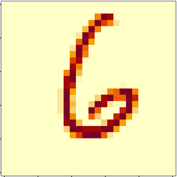

3. Make a PCA, choice wether to scale or not.

myPCA <- select(mnist, -instance) %>% 
  PCA(graph = FALSE, scale.unit = FALSE, quali.sup = 1, ncp = 500)

4. Make the usual diagnostic plots (screeplot, individual, variable) for the first axes, and comment.

Be careful with the biplot on unscaled PCA.

fviz_eig(myPCA, ncp = 50)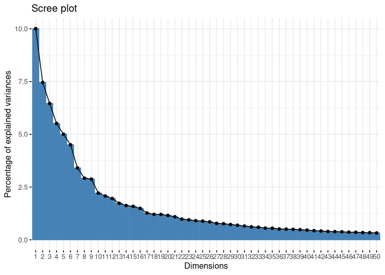

fviz_pca_ind(myPCA, habillage = "label")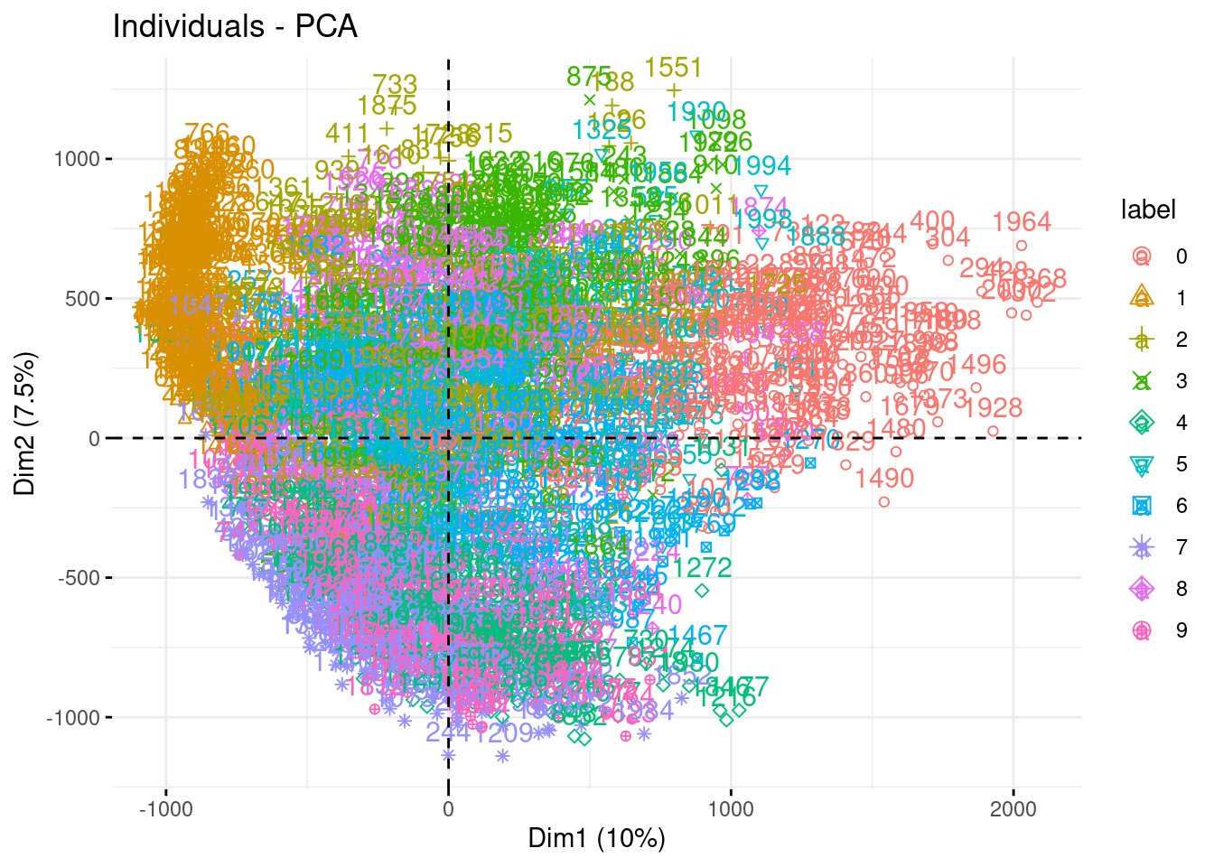

fviz_pca_ind(myPCA, habillage = "label", axes = c(1,3))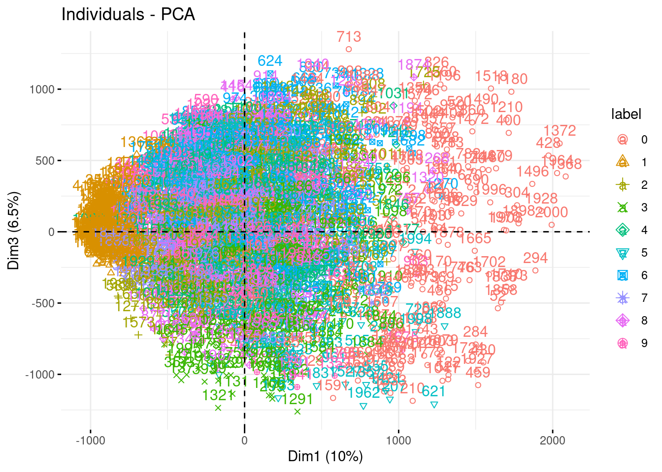

fviz_pca_ind(myPCA, habillage = "label", axes = c(2,3))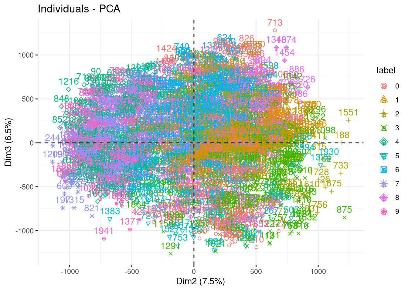

fviz_pca_var(myPCA, col.var = 'cos2', select.var = list(contrib = 30))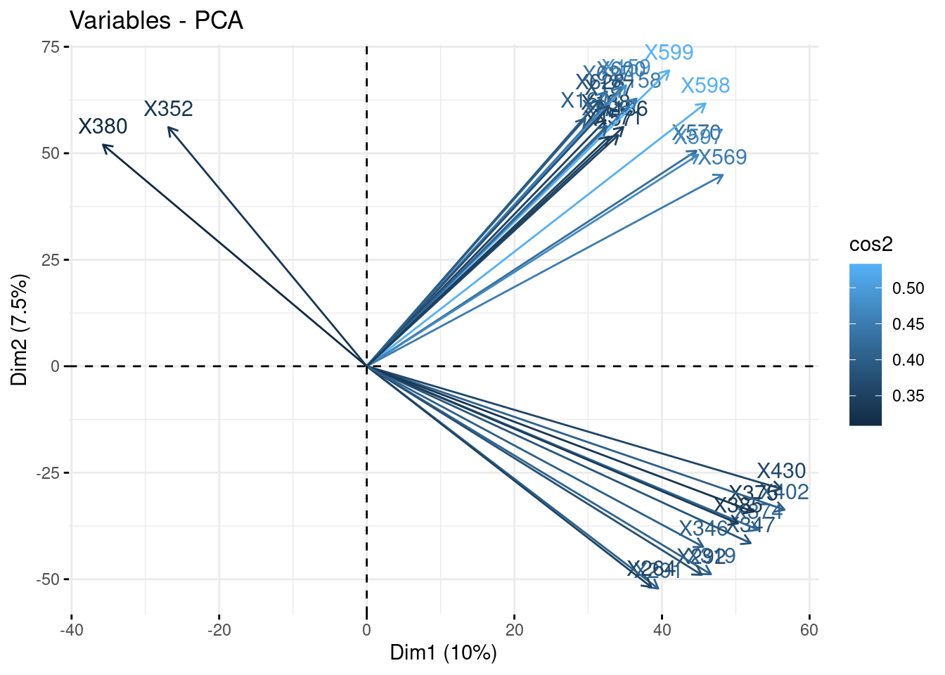

npc <- select(mnist, -instance, -label) %>% replace(is.na(.), 0) %>% 
    as.matrix() %>% scale(TRUE, FALSE) %>% 
    estim_ncp(ncp.max = 500, scale = FALSE) 
plot(npc$criterion, type = "l", xlab = 'number of component', ylab = 'GCV')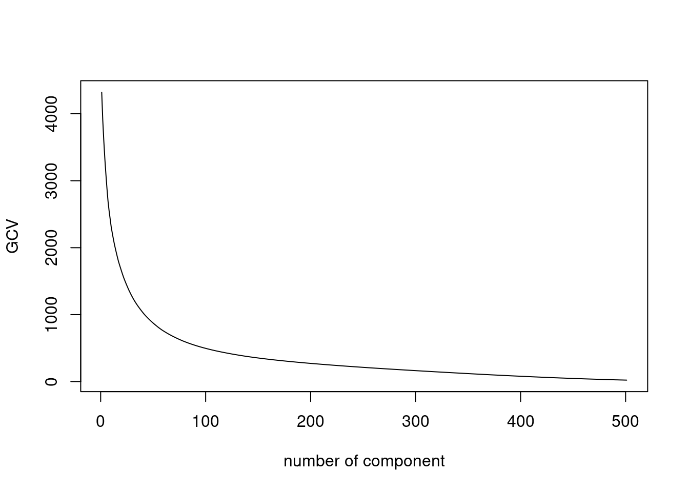

5. Write a function to reconstruct an image with two argument: \(i\) (an instance) \(k\) (the number of component used).

## Continuous attributes
X <- select(mnist, -label, -instance) %>%  scale(TRUE, FALSE)

## Loadings/rotation matrix
U <- eigen(cov(X))$vectors

## Function for projection
proj_data <- function(k, i) {
  X[i, , drop = FALSE] %*% U[, 1:k, drop = FALSE] %*% t(U[, 1:k, drop = FALSE]) %>% 
    as.numeric()
}

6. Plot the reconstructed image for various value of \(k\)

Let us pick 9 pictures randomly, and define a sequence for the number of axes used to perform the reconstruction (up to a perfect reconstruction).

nb_samples <- 9
samples <- sample.int(1000, nb_samples)
nb_axis <- c(1, 2, 10, 20, 100, ncol(X))

Now here is a solution in ‘base’ R

cases <- expand.grid(nb_axis, samples)
## list of approximated images (stored as vectors)
approx <- mapply(proj_data, cases[, 1], cases[, 2], SIMPLIFY = FALSE)

  
par(mfrow=c(nb_samples, length(nb_axis)), mar = c(0.1,0.1,0.1,0.1))
silent <- utils::capture.output(lapply(approx, plot_picture))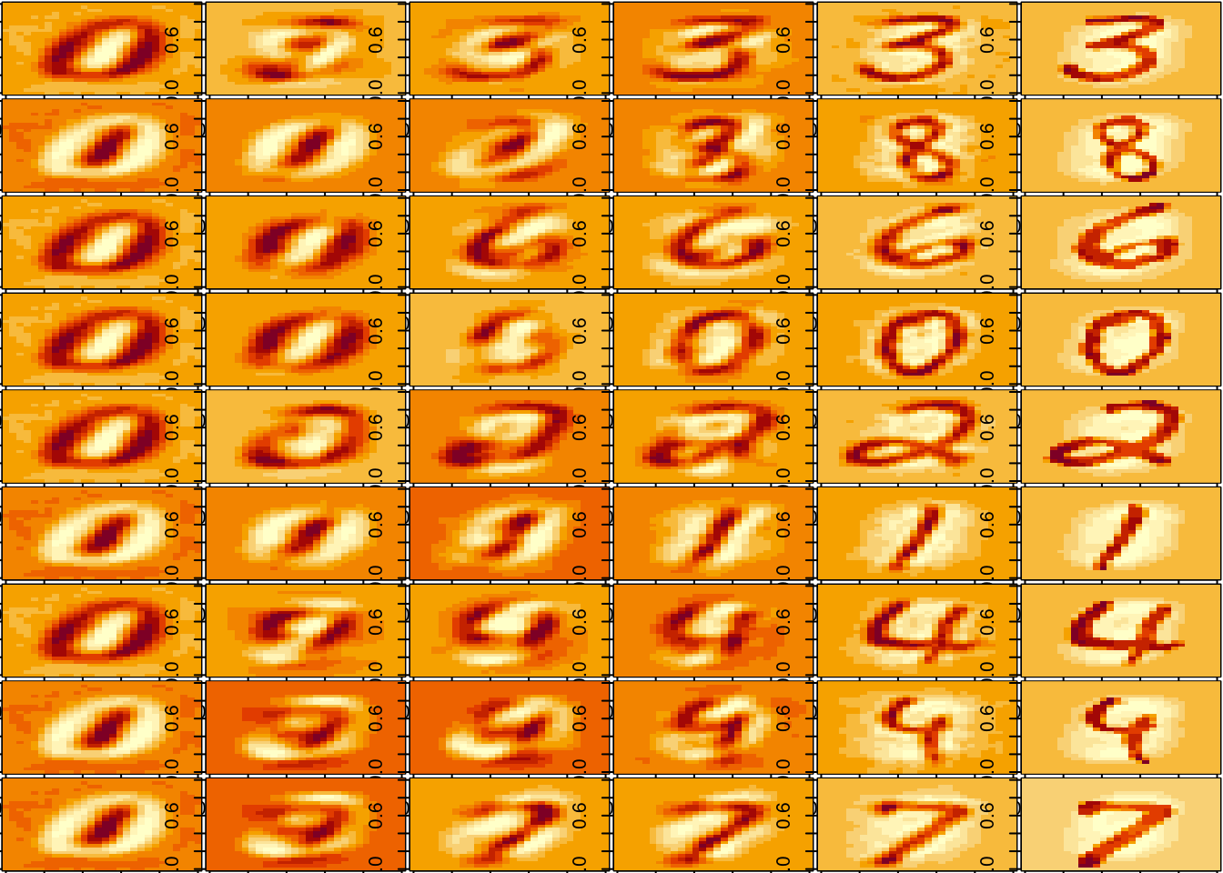

And another solution using {ggplot}.

## fancy ggplot output
labels <- mnist %>% dplyr::filter(instance %in% samples) %>% pull(label)
instances <- mnist %>% dplyr::filter(instance %in% samples) %>% pull(instance)
approx_tibble <- do.call(rbind, approx) %>% as_tibble() %>% 
  add_column(nb_axis = rep(nb_axis, length(samples)), .before = 1) %>% 
  add_column(label = rep(labels, each = length(nb_axis)), .before = 1) %>% 
  add_column(instance = rep(instances, each = length(nb_axis)), .before = 1)

## Warning: The `x` argument of `as_tibble.matrix()` must have unique column names if `.name_repair` is omitted as of tibble 2.0.0.
## Using compatibility `.name_repair`.

approx_tibble %>% 
   gather(pixel, value, -label, -instance, -nb_axis) %>%
   tidyr::extract(pixel, "pixel", "(\\d+)", convert = TRUE) %>%
   mutate(pixel = pixel - 2,
          x = pixel %% 28,
          y = 28 - pixel %/% 28) %>% 
   ggplot(aes(x, y, fill = value)) +
   geom_tile() +
   facet_grid(label ~ nb_axis)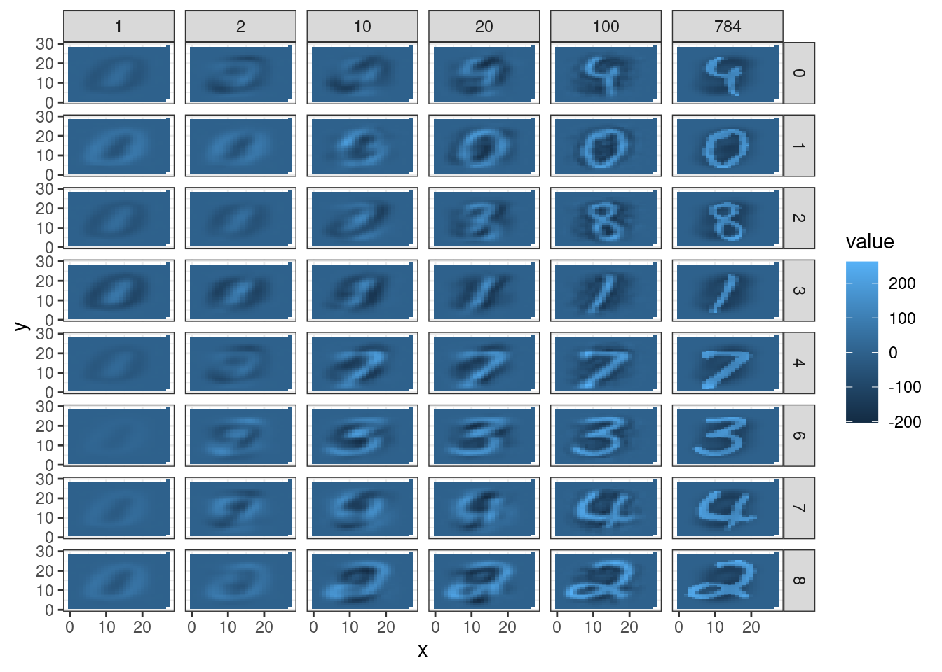

Decathlon: analysing performance between athletes

Courtesy of Julie Josse, thanks!

Data description

This dataset contains the results of decathlon events during two athletic meetings which took place one month apart in 2004: the Olympic Games in Athens (23 and 24 August), and the Decastar 2004 (25 and 26 September). For both competitions, the following information is available for each athlete: performance for each of the 10 events, total number of points (for each event, an athlete earns points based on performance; here the sum of points scored) and final ranking. The events took place in the following order: 100 meters, long jump, shot put, high jump, 400 meters (first day) and 110 meter hurdles, discus, pole vault, javelin, 1500 meters (second day). Nine athletes participated to both competitions. We would like to obtain a typology of the performance profiles.

The data are distributed with {FactoMineR}

library(FactoMineR)
data("decathlon")

Questions

1. Inspect the data set with the following commands:
2. Explain the interest of centering and scaling the data. Could you spotlight outstanding athletes ? Which inequality are you using?
3. Explain your choices for the active and illustrative variables/individuals and perform the PCA on this data set.
4. Comment

• the correlation between the 100 m and long.jump
• the correlation between long.jump and Pole.vault
• can you describe the athlete Casarsa?
• the proximity between Sebrle and Clay
• the proximity between Schoenbeck and Barras

5. In which trials those who win the decathlon perform the best? Could we say that the decathlon trials are well selected?
6. Compare and comment the performances during both events: Decastar and Olympic. Could we conclude on the differences? Plot Confidence ellipses
7. Select the number of dimensions with the function estim_npc.

Solution (compulsive click forbidden!)

1. Inspect the data set with the following commands:
2. Explain the interest of centering and scaling the data. Could you spotlight outstanding athletes?

When the data are standardized, it is possible to compare two variables with different units and to say sentences such as “Paul is more remarkable by his height than John is by is weight”. When looking at the standardized data, we can look for the values greater or smaller than 2 for instance. We are refering to Bienaymé-Tchebychev which states that 25% of the observations will be at 2 standard deviation from their means. If we consider Gaussian data, we can refine this inequality and consider know that 4.5 % of the observations are greater than 2 in absolute value. Sebrle value for Javeline is 2.528251350 meaning that he is far above average.

The aim of conducting PCA on this dataset is to determine profiles for similar performances: are there any athletes who are better at endurance events or those requiring short bursts of energy, etc? And are some of the events similar? If an athlete performs well in one event, will he necessarily perform well in another?

3. Explain your choices for the active and illustrative variables/individuals and perform the PCA on this data set.

decathlon_PCA <- PCA(decathlon, quanti.sup = c(11,12) , quali.sup = 13)

## Warning: ggrepel: 1 unlabeled data points (too many overlaps). Consider
## increasing max.overlaps

fviz_eig(decathlon_PCA)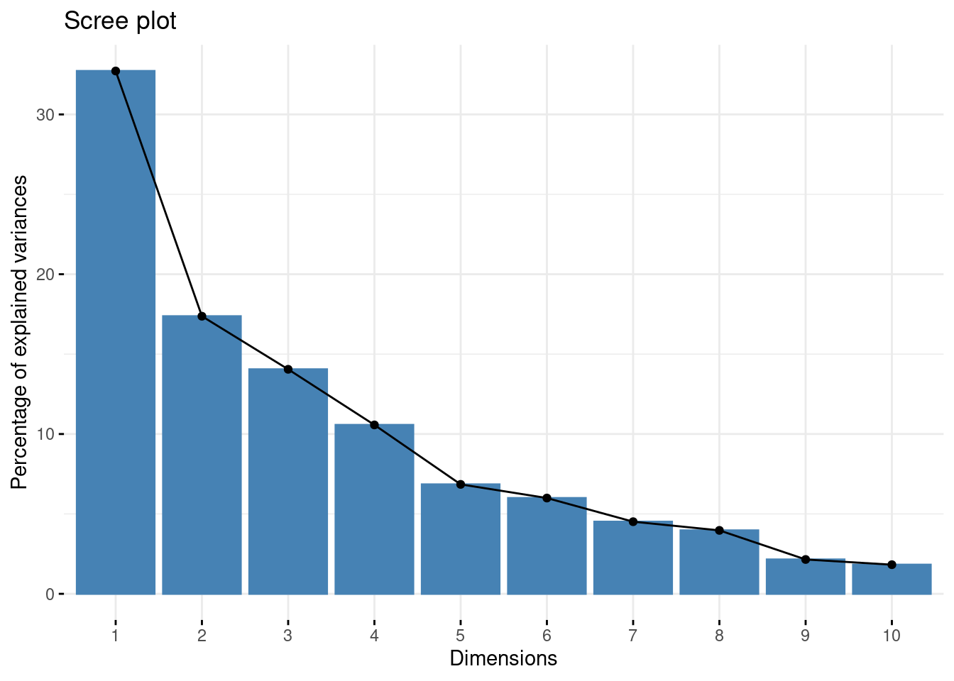

fviz_pca_ind(decathlon_PCA, axes = c(3, 4))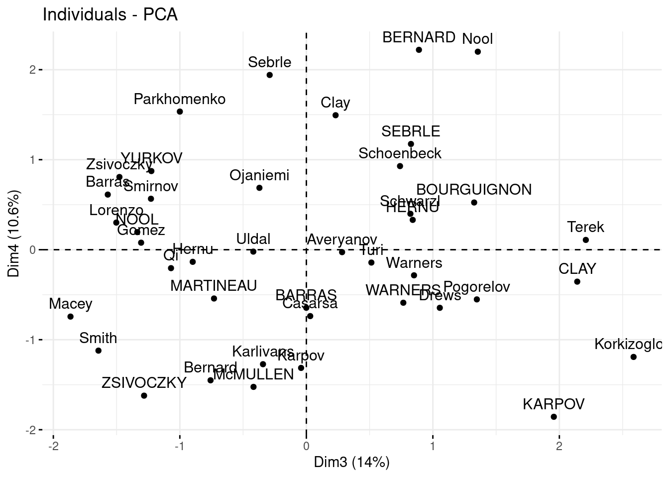

fviz_pca_var(decathlon_PCA, axes = c(3, 4))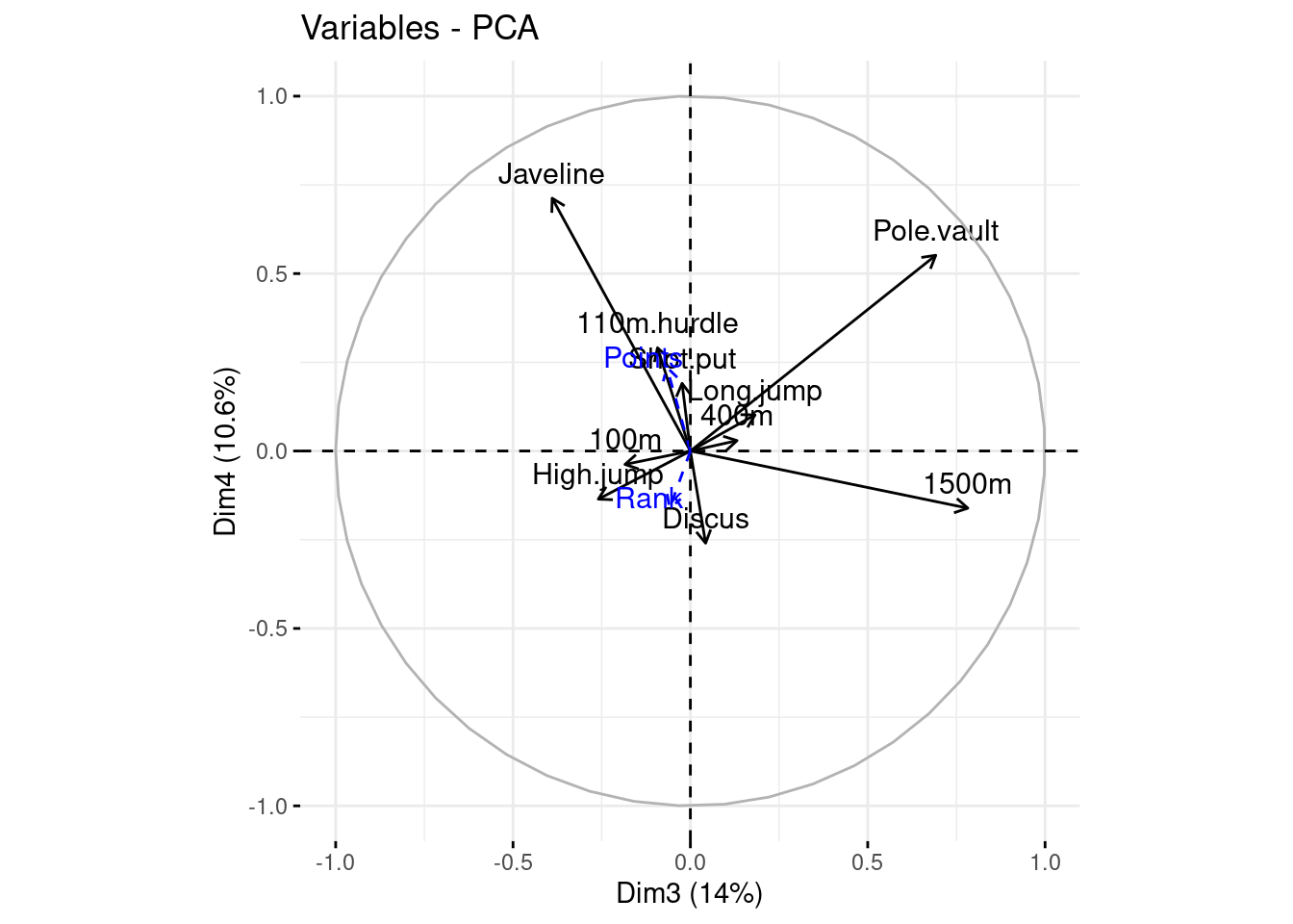

To obtain a typology of the athletes based on their performances for the 10 decathlon events, such as “two athletes are close as they have similar performance profiles”, the distances between two athletes are defined on the basis of their performances in the 10 events. Thus, only the performance variables are considered active; the other variables (number of points, rank, and competition) are supplementary. Here, the athletes are all considered as active individuals.

4. Comment:

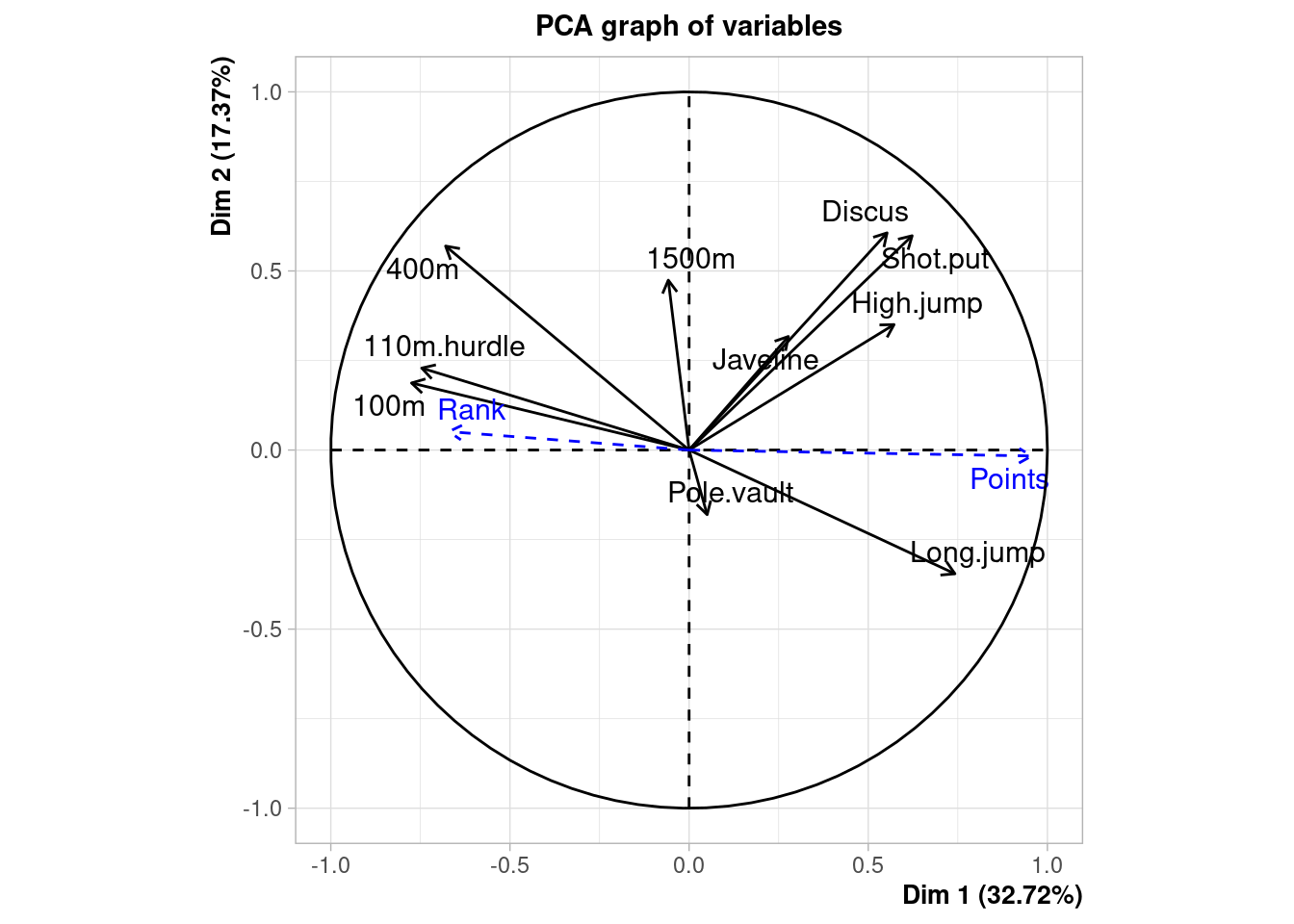
• the correlation between the 100 m and long.jump

The 100m and long.jump are negatively correlated: therefore, an athlete who runs 100 meters quickly will generally jump a long way. The variables 100m, 400m, and 110m hurdles are positively correlated, that is, some athletes perform well in all four events while others do not.

• the correlation between long.jump and Pole.vault

Since long.jump is well represented in the first plan and Pole.vault is not, we can deduce that long.jump and Pole.vault are approximately orthogonal, meaning that the corresponding variables are roughly uncorrelated. Overall, the variables relating to speed are negatively correlated with the first principal component while the variables shot put and long jump are positively correlated with this component. The coordinates of these active variables can be found in the object which also gives the representation quality of the variables (cosine squared) and their contributions to the construction of the components.

Bourguignon and Karpov have very different performance profiles since they are opposed according to the main axis of variability.

• can you describe the athlete Casarsa?

Casarsa is located on the top left corner. The first dimension is highly correlated with the number of points: this indicates that he does not have a large number of points. The second dimension is correlated with the Shot.put, High.jump and Discus. This indicates that Casarsa had good results in these three sports. Remember that the second dimension is calculated orthogonally to the first. So Casarsa has good results in these three sports compared to other “bad” athletes.

• the proximity between Sebrle and Clay

Sebrle and Clay are close to one another and both far from the center of gravity of the cloud of points. The quality of their projection is therefore good, and we can be certain that they are indeed close in the original space. This means that they have similar profiles in their results across all sports events.

• the proximity between Schoenbeck and Barras

Schoenbeck and Barras are close to one another but they are also close to the center of gravity of the cloud of points. When looking at their cos2 they are not well projected, We cannot interpret their distance based on this plot only.

5. In which trials those who win the decathlon perform the best? Could we say that the decathlon trials are well selected?

The supplementary variable “number of points” is almost collinear to the first principal component. Therefore, the athletes with a high number of points are particularly good in the trials correlated with the first principal component. Those who win the decathlon perform the best in 100m, 110m hurdles and long jump. This means that the ranking of the decathlon is governed by those three sports.

6. Compare and comment the performances during both events: Decastar and Olympic, by ploting confidence ellipses.

plotellipses(decathlon_PCA)

## Warning: ggrepel: 1 unlabeled data points (too many overlaps). Consider
## increasing max.overlaps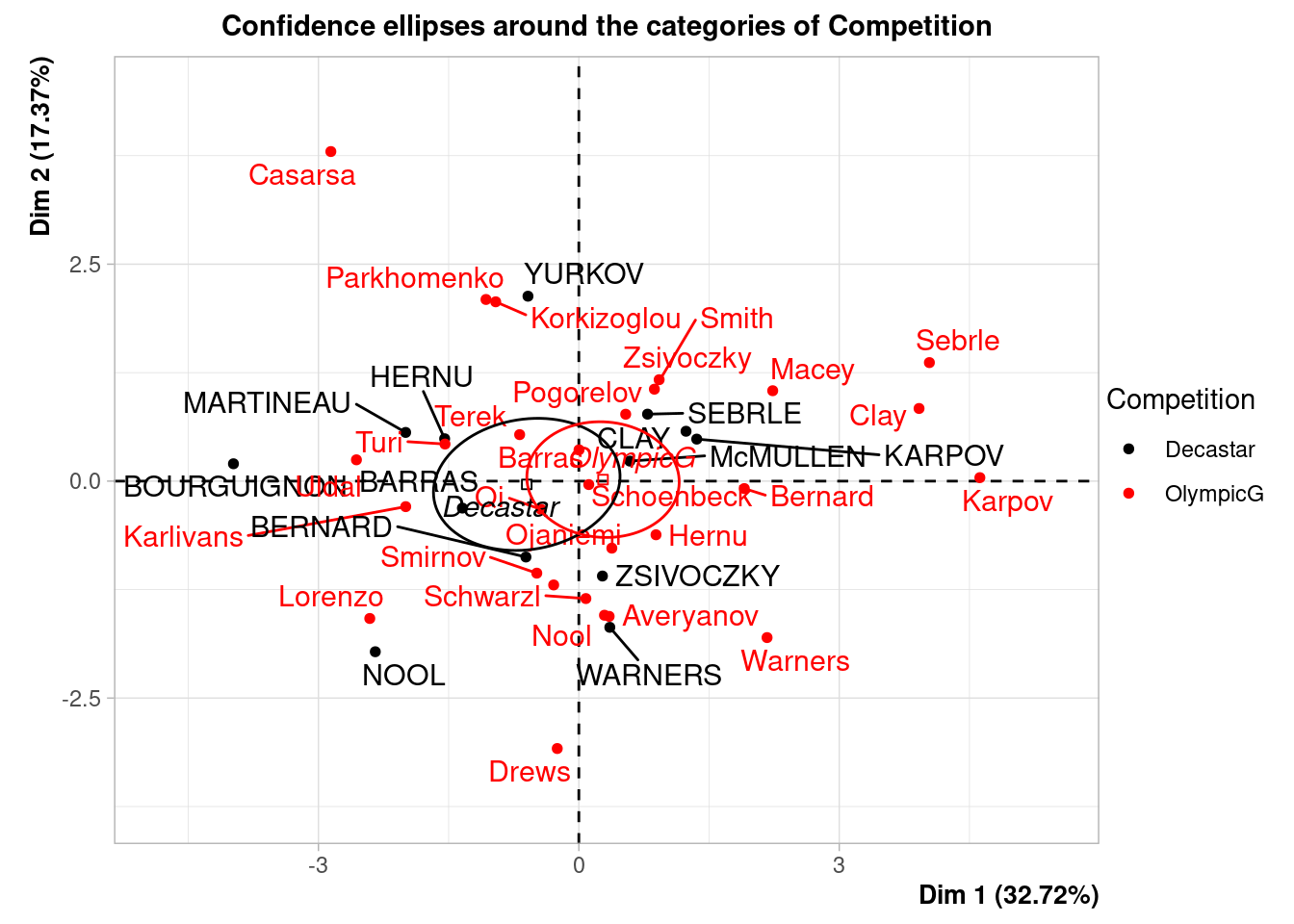

7. Select the number of dimensions with the function estim_npc.

plot(estim_ncp(decathlon[, 1:10])$criterion, type = "l", xlab = "number of axis", ylab = "GCV")