Generating Gaussian data from a Graphical Model with SBM structure

Preliminaries

library(rggm)
library(igraph)
library(corrplot)
library(Matrix)

Generating a graph under the stochastic bloc model

SBM parameters

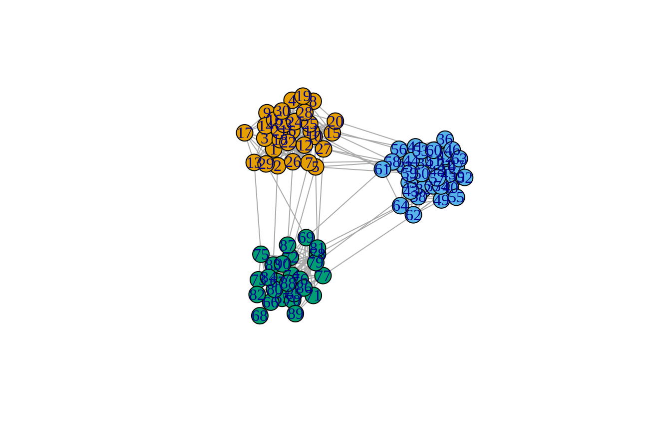
We consider in the following an undirect network \(\mathcal{G}\) with 100 nodes splitted into 3 blocks with community-like connectivity:

nNodes  <- 90
blockProp <- c(1/3, 1/3, 1/3)   # group proportions
nbBlock   <- length(blockProp) # number of blocks
connectParam <- diag(.4, nbBlock) + 0.01 # connectivity matrix: affiliation network

Sampling under the SBM

The function rSBM sample a binary network under the SBM. Let us try the aformentioned set of parameters:

## Graph Sampling
mySBM <- rSBM(nNodes, connectParam, blockProp)
## Graph plotting
plot(mySBM, vertex.color = V(mySBM)$memberships)

Adding weights to the edges

In rggm, the user can add some random weights to the edges of an existing SBM. Those weigths are drawn under a predefined distribution (only “gaussian” and “poisson” are implemented at the moment) the parameters of which are defined blocwise

Gaussian weights

We consider for instance Gaussian weights in this piece of code:

## Sampling Gaussian weights
mu_within   <- 4 ; sigma_within  <- .5
mu_between  <- 2 ; sigma_between <- .5
theta <- list()
theta$mu    <- matrix(mu_between   , nbBlock, nbBlock); diag(theta$mu)    <- mu_within    # means
theta$sigma <- matrix(sigma_between, nbBlock, nbBlock); diag(theta$sigma) <- sigma_within # sd

mySBM_Gaussian <- rWeightSBM(mySBM, "gaussian", theta)
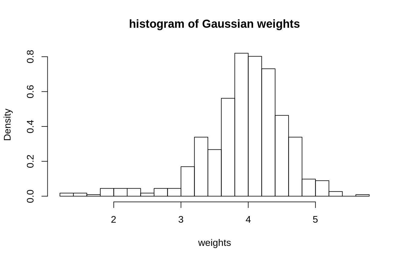
hist(E(mySBM_Gaussian)$weight,  breaks = sqrt(gsize(mySBM_Gaussian)), freq = FALSE, xlab = "weights", main = "histogram of Gaussian weights")

Others weights: Poisson or Laplace

At the moment, one could add Poisson or Laplace weigths as an alternative to binary or Gaussian weights on the edges:

## Sampling Laplace weights
m_within   <- 4 ; s_within  <- .5
m_between  <- 2 ; s_between <- .5
theta <- list()
theta$m <- matrix(m_between, nbBlock, nbBlock); diag(theta$m) <- m_within # location parameter
theta$s <- matrix(s_between, nbBlock, nbBlock); diag(theta$s) <- s_within # scale parameters

mySBM_Laplace <- rWeightSBM(mySBM, "laplace", theta)

## Sampling Poisson weights
lambda_within   <- 4
lambda_between  <- 1
theta <- list()
theta$lambda <- matrix(lambda_between, nbBlock, nbBlock); diag(theta$lambda) <- lambda_within # mean/variance parameter
#'
mySBM_Poisson <- rWeightSBM(mySBM, "poisson", theta)

par(mfrow = c(1,2))
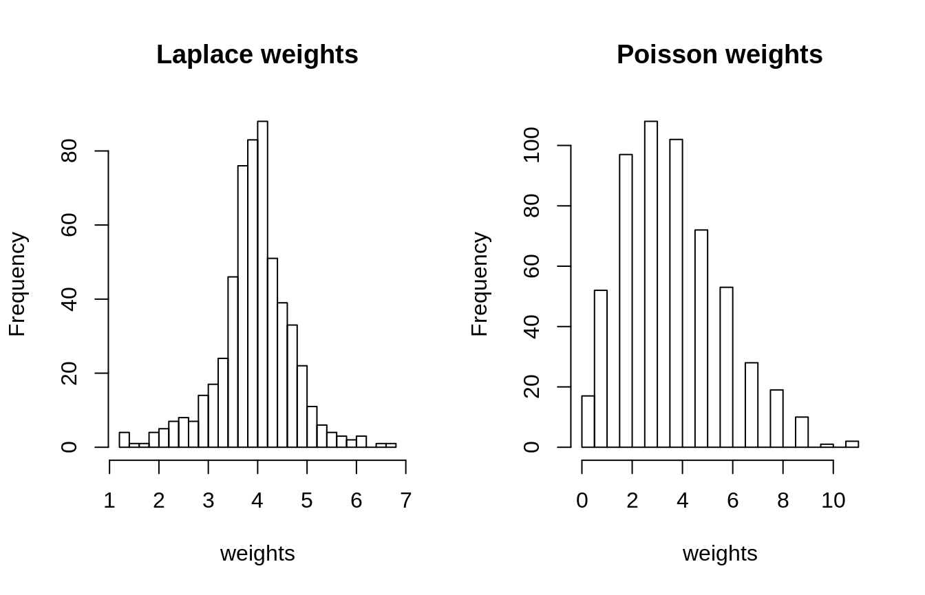
hist(E(mySBM_Laplace)$weight,  breaks = sqrt(gsize(mySBM_Laplace)), xlab = "weights", main = "Laplace weights")
hist(E(mySBM_Poisson)$weight,  breaks = sqrt(gsize(mySBM_Poisson)), xlab = "weights", main = "Poisson weights")

Drawing multivariate Gaussian observations faithful to a the graph

Consider the multivariate Gaussian model \[ X \sim \mathcal{N}(\mathbf{m}, \boldsymbol\Sigma), \qquad \text{with } \boldsymbol\Omega = \boldsymbol\Sigma^{-1} \text{ the precision matrix}. \]

We would like to drawn observation of the Gaussian vector \(X\) such that \(\boldsymbol\Omega\) has a sparsity pattern faithful to the orginal graph \(\mathcal{G}\) generated under the SBM.

Constructing the precision matrix and the variance-covariance

The function graph2prec allows one to build a precision matrix \(\boldsymbol\Omega\) faitful to the original graph, that is, with a sparsity pattern reflecting the graphical model of the SBM generated above. To this end, we rely on the Laplacian matrix which is set diagonal dominant by increasing iteratively its diagonal. Note that when the graph is weighted, the weighted Laplacian is used.

An optional argument allows to fix the conditional variance a priori¹. This argument allows the user to indirectly tune the variances in the variance-covariance matrix \(\boldsymbol\Sigma\).

For instance, if we want to fix the conditional variances to 1 (and thus get variances all equal to 1),

Omega <- graph2prec(mySBM_Gaussian, cond_var = rep(1, gorder(mySBM)))

The variance-covariance \(\boldsymbol\Sigma\) is then obtain be inversion, since \(\boldsymbol\Omega\) is guaranted to be strictly positive-definite.

Sigma <- solve(Omega)

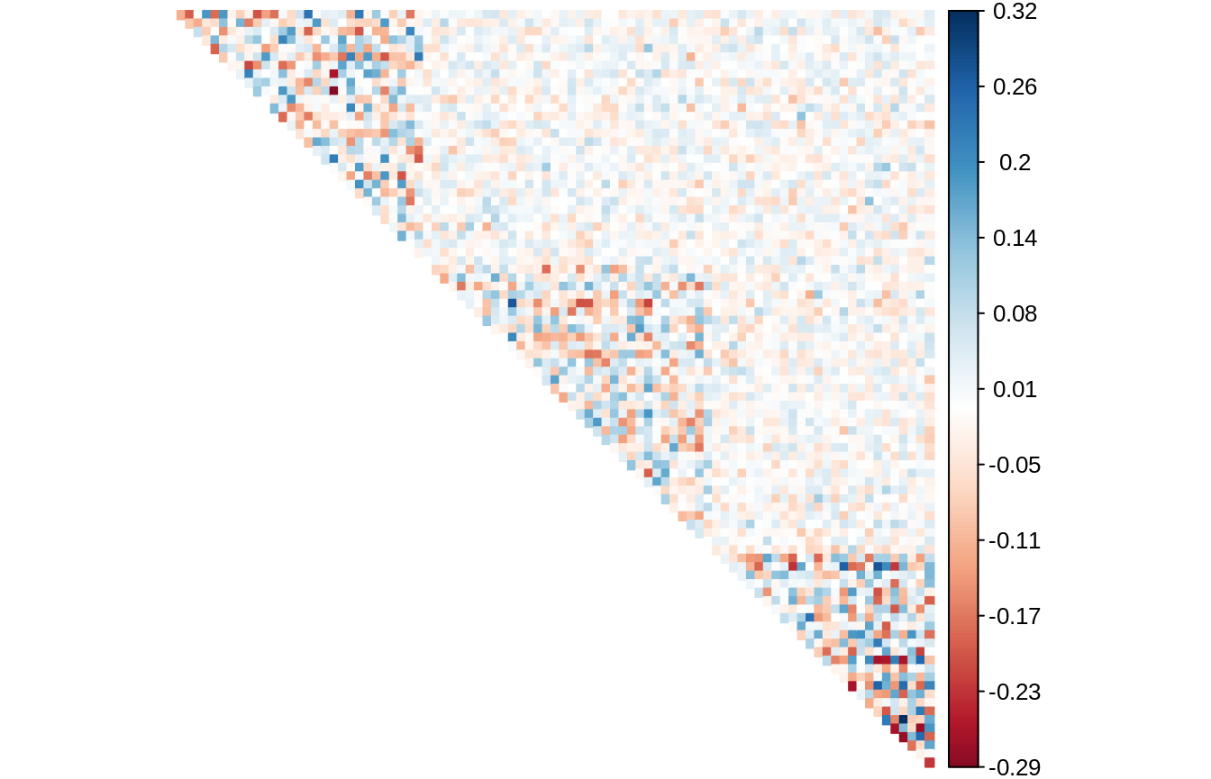
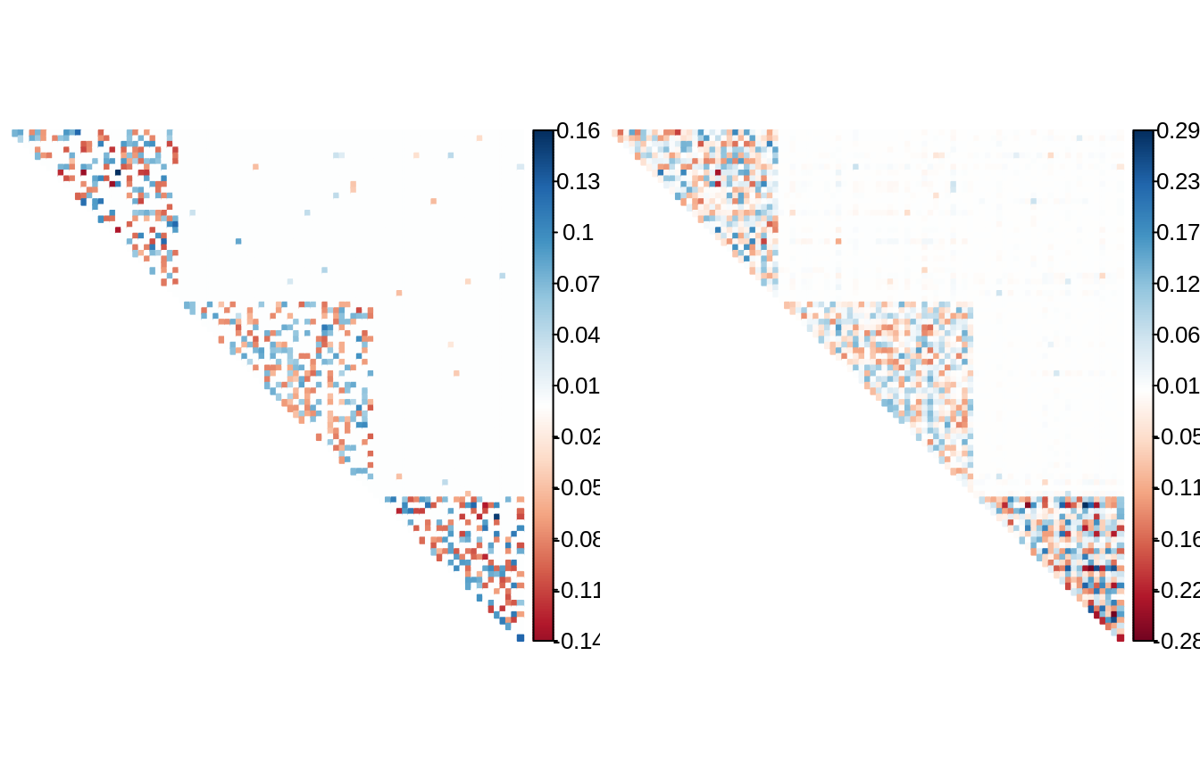
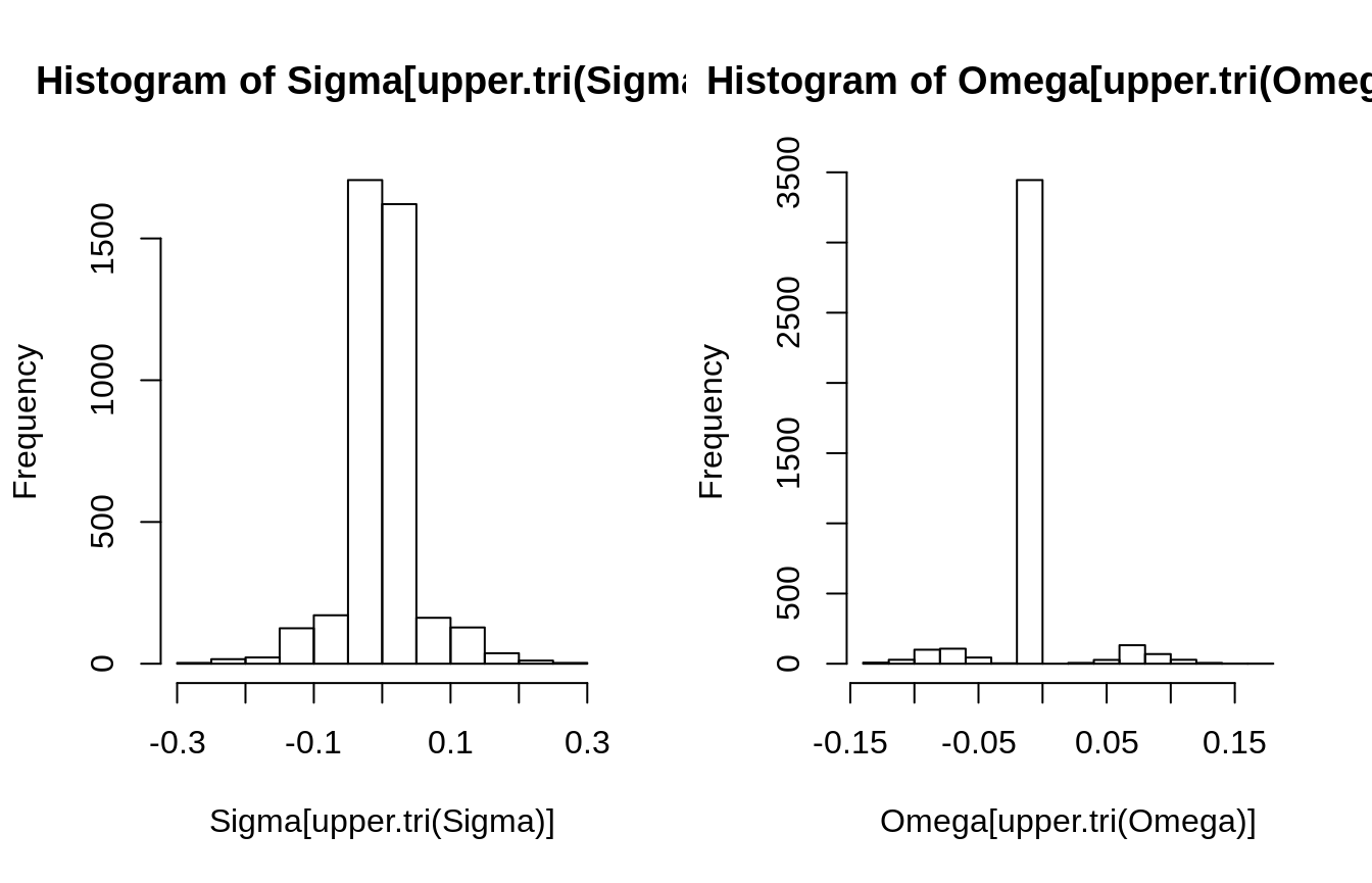
The corresponding matrices exhibit the expected strong block-diagonal structure of the original affilitation graph.

par(mfrow = c(1,2))
corrplot(as.matrix(Omega), is.corr = FALSE, tl.pos = "n", method = 'color', type = "upper", diag = FALSE)
corrplot(as.matrix(Sigma), is.corr = FALSE, tl.pos = "n", method = 'color', type = "upper", diag = FALSE)

hist(Sigma[upper.tri(Sigma)])
hist(Omega[upper.tri(Omega)])

Gaussian Observations

n <- 1000
means <- rep(0, ncol(Sigma))
X <- rmgaussian(n, means, Sigma)
Sigma_hat <- cov(as.matrix(X))
corrplot(Sigma_hat, is.corr = FALSE, method = 'color', type = "upper", diag = FALSE, tl.pos = "n")

TO BE CONTINUED -> signal seems a bit weak…

conditional variances are equal to the inverse of the diagonal in a precision matrix↩

01 April, 2020