Fit a linear model with infinity-norm plus ridge-like regularization

Adjust a linear model penalized by a mixture of a (possibly weighted) \(\ell_\infty\)-norm (bounding the magnitude of the parameters) and a (possibly structured) \(\ell_2\)-norm (ridge-like). The solution path is computed at a grid of values for the infinity-penalty, fixing the amount of \(\ell_2\) regularization. See details for the criterion optimized.

Usage

bounded.reg(
  x,
  y,
  lambda1 = NULL,
  lambda2 = 0.01,
  penscale = rep(1, ncol(x)),
  struct = Matrix::Diagonal(ncol(x), 1),
  intercept = TRUE,
  normalize = TRUE,
  nlambda1 = ifelse(is.null(lambda1), 100, length(lambda1)),
  minratio = ifelse(nrow(x) <= ncol(x), 0.01, 1e-04),
  maxfeat = ifelse(lambda2 < 0.01, min(nrow(x), ncol(x)), min(4 * nrow(x), ncol(x))),
  control = list()
)

Arguments

x

matrix of features, possibly sparsely encoded (experimental). Do NOT include intercept. When normalized os TRUE, coefficients will then be rescaled to the original scale.

y

response vector.

lambda1

sequence of decreasing \(\ell_1\)-penalty levels. If NULL (the default), a vector is generated with nlambda1 entries, starting from a guessed level lambda1.max where only the intercept is included, then shrunken to minratio*lambda1.max.

lambda2

real scalar; tunes the \(\ell_2\) penalty in the Elastic-net. Default is 0.01. Set to 0 to recover the Lasso.

penscale

vector with real positive values that weight the \(\ell_1\)-penalty of each feature. Default set all weights to 1.

struct

matrix structuring the coefficients, possibly sparsely encoded. Must be at least positive semidefinite (this is checked internally). If NULL (the default), the identity matrix is used. See details below.

intercept

logical; indicates if an intercept should be included in the model. Default is TRUE.

normalize

logical; indicates if variables should be normalized to have unit L2 norm before fitting. Default is TRUE.

nlambda1

integer that indicates the number of values to put in the lambda1 vector. Ignored if lambda1 is provided.

minratio

minimal value of \(\ell_1\)-part of the penalty that will be tried, as a fraction of the maximal lambda1 value. A too small value might lead to unstability at the end of the solution path corresponding to small lambda1 combined with \(\lambda_2=0\). The default value tries to avoid this, adapting to the '\(n<p\)' context. Ignored if lambda1 is provided.

maxfeat

integer; limits the number of features ever to enter the model; i.e., non-zero coefficients for the Elastic-net: the algorithm stops if this number is exceeded and lambda1 is cut at the corresponding level. Default is min(nrow(x),ncol(x)) for small lambda2 (<0.01) and min(4*nrow(x),ncol(x)) otherwise. Use with care, as it considerably changes the computation time.

control

list of argument controlling low level options of the algorithm –use with care and at your own risk– :

verbose: integer; activate verbose mode –this one is not too risky!– set to 0 for no output; 1 for warnings only, and 2 for tracing the whole progression. Default is 1. Automatically set to 0 when the method is embedded within cross-validation or stability selection.
timer: logical; use to record the timing of the algorithm. Default is FALSE.
maxiter the maximal number of iteration used to solve the problem for a given value of lambda1. Default is 500.
method a string for the underlying solver used. Either "quadra" or "fista". Default is "quadra".
threshold a threshold for convergence. The algorithm stops when the optimality conditions are fulfill up to this threshold. Default is 1e-7 for "quadra" and 1e-2 for the first order methods.
monitor indicates if a monitoring of the convergence should be recorded, by computing a lower bound between the current solution and the optimum: when '0' (the default), no monitoring is provided; when '1', the bound derived in Grandvalet et al. is computed; when '>1', the Fenchel duality gap is computed along the algorithm.

Value

an object with class QuadrupenFit.

an object with class BoundedRegressionFit, inheriting from QuadrupenFit.

Note

The optimized criterion is

β^hat_λ₁,λ₂ = argmin_β 1/2 RSS(&beta) + λ₁ | D β |_∞ + λ/2 ₂ β^T S β, where \(D\) is a diagonal matrix, whose diagonal terms are provided as a vector by the penscale argument. The \(\ell_2\) structuring matrix \(S\) is provided via the struct argument, a positive semidefinite matrix (possibly of class Matrix).

Note that the quadratic algorithm for the bounded regression may become unstable along the path because of singularity of the underlying problem, e.g. when there are too much correlation or when the size of the problem is close to or smaller than the sample size. In such cases, it might be a good idea to switch to the proximal solver, slower yet more robust. This is the strategy automatically adopted in code, that will send a warning in verbose mode while switching the method to 'fista' and keep on optimizing on the remainder of the path.

Singularity of the system can also be avoided with a larger \(\ell_2\)-regularization, via lambda2, or a "not-too-small" \(\ell_\infty\) regularization, via a larger 'minratio' argument.

Examples

## Simulating multivariate Gaussian with blockwise correlation
## and piecewise constant vector of parameters
beta <- rep(c(0,1,0,-1,0), c(25,10,25,10,25))
cor <- 0.75
Soo <- toeplitz(cor^(0:(25-1))) ## Toeplitz correlation for irrelevant variables
Sww  <- matrix(cor,10,10) ## bloc correlation between active variables
Sigma <- Matrix::bdiag(Soo,Sww,Soo,Sww,Soo)
diag(Sigma) <- 1
n <- 50
x <- as.matrix(matrix(rnorm(95*n),n,95) %*% chol(Sigma))
y <- 10 + x %*% beta + rnorm(n,0,10)

## Infinity norm without/with an additional l2 regularization term
## and with structuring prior
labels <- rep("irrelevant", length(beta))
labels[beta != 0] <- "relevant"
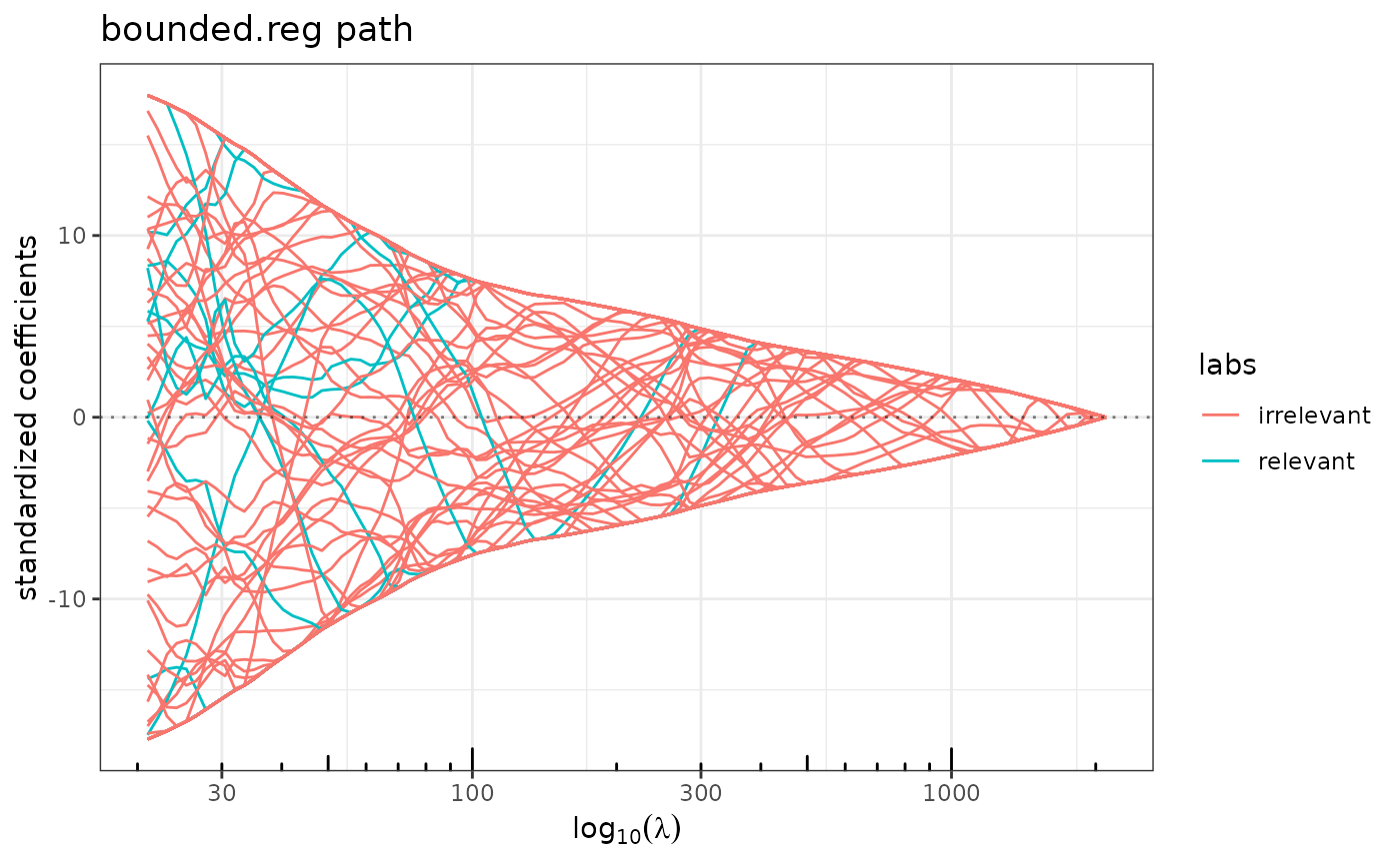
plot(bounded.reg(x,y,lambda2=0) , label=labels) ## a mess

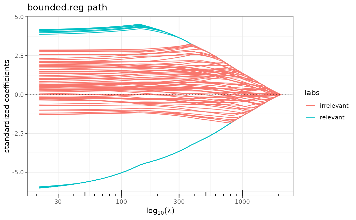
plot(bounded.reg(x,y,lambda2=10), label=labels) ## good guys are at the boundaries

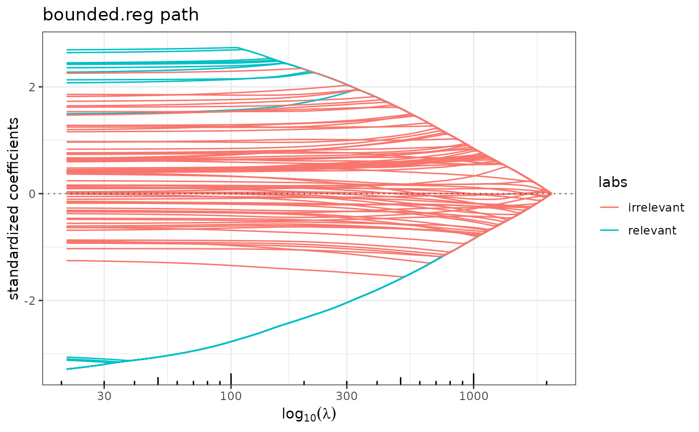plot(bounded.reg(x,y,lambda2=10,struct=solve(Sigma)), label=labels) ## even better